Classifying Smartphone Apps with Keras
Overview
Teaching: 20 min
Exercises: 40 minQuestions
How do we build a neural network on KERAS to perform multi-class classification?
How do we monitor the progress of neural-network training?
How do we set up appropriate hyperparameters?
Objectives
Understanding how to build a general neural network with KERAS.
Understanding how to tune the hyperparameters based on the results.
Prior to this episode, we focused on an extremely simple problem:
a binary classification task using the sherlock_2apps (“2-apps”) data.
Certainly, this is a very basic problem;
real-world problems have much richer complexities.
Beginning from this episode, we will use a richer subset of Sherlock’s
Applications.csv to build a classifier to distinguish nearly 20 smartphone apps.
As in the previous episode, we will build simple neural networks with KERAS
(using all the essential building blocks of a neural network introduced in that
episode) and quantify their performance metrics. As we progress, we will
introduce additional techniques that are helpful in practical ML modeling.
Along the way, we will be guided to answer the following questions:
-
How far can we push the accuracy of a neural network model for smartphone app classification?
-
As a bonus exercise, what will the accuracies be if we build decision tree and logistic regression models to perform the same classification task?
Loading Required Python Libraries and Objects
Please make sure that the necessary libraries and objects are loaded into your environment:
import os
import sys

import pandas as pd
import numpy as np
import matplotlib.pyplot as plt

# Tools for machine learning:
import sklearn
from sklearn import preprocessing
from sklearn.model_selection import train_test_split
# for evaluating model performance
from sklearn.metrics import accuracy_score, confusion_matrix
# classic machine learning models
from sklearn.linear_model import LogisticRegression
from sklearn.tree import DecisionTreeClassifier

# Tools for deep learning:
import tensorflow as tf
import tensorflow.keras as keras

# Import key Keras objects
from tensorflow.keras.models import Sequential
from tensorflow.keras.layers import Dense
from tensorflow.keras.optimizers import Adam
These are the same imports used at the beginning of the previous episode on binary classification. you start with a fresh Python session in this episode to avoid any confusion caused by using a different dataset.
The sherlock_18apps Dataset
The dataset used for this episode is the “18-apps” dataset, a significantly more diverse subset of the SherLock dataset that includes nearly 20 apps. Not only are there more classes (apps), but the dataset also contains more features. As with the 2-apps counterpart, the rows stored in this table were generated by periodically measuring the resource (CPU, memory, network, input/output) utilization stats for the individual apps. The table below presents the features of this dataset and offers a brief explanation of each:
| No | Feature | Data Type | Meaning |
|---|---|---|---|
| 0 | CPU_USAGE |
float | Instantaneous percent utilization of CPU |
| 1 | UidRxBytes |
int | Number of bytes received by this app via network |
| 2 | UidRxPackets |
int | Number of network packets received by this app |
| 3 | UidTxBytes |
int | Number of bytes transmitted (sent) by this app via network |
| 4 | UidTxPackets |
int | Number of network packets received transmitted by this app |
| 5 | cutime |
int | (Linux) Amount of CPU time spent in “user-mode” by the spawned & waited on child process |
| 6 | guest_time |
int | (Linux) Amount of CPU time spent running a virtual CPU |
| 7 | importance |
int | (Android) The relative importance of this app, as set by the Android system |
| 8 | lru |
int | (Android) An additional ordering within a particular Android importance category |
| 9 | num_threads |
int | (Linux) Number of threads in this app |
| 10 | otherPrivateDirty |
int | (Android) Amount of dirty memory (i.e. written by this app), in units of kiB |
| 11 | priority |
int | (Linux) The process’s priority in terms of CPU scheduling policy. |
| 12 | rss |
int | (Linux) The amount of memory (RAM) actually occupied by this app, in units of kiB |
| 13 | state |
char | (Linux) The state of the app’s process (Sleeping, Running, Busy I/O (D), Zombie |
| 14 | stime |
int | (Linux) Amount of CPU time spent in “system-mode” by the app |
| 15 | utime |
int | (Linux) Amount of CPU time spent in “user-mode” by the app |
| 16 | vsize |
int | (Linux) Amount of virtual memory allocated for the app, in units of bytes |
| 17 | cminflt |
int | (Linux) Number of minor page faults of the spawned & waited child process |
(Source: Sherlock Dataset Data Field Description, version 2.4.1 by the SherLock team at BGU.) The explanations in the “meaning” field above are terse; they do not precisely explain everything we need to know about these fields. Those marked with “(Linux)” are tracked and reported by the operating system (Linux OS), those with “(Android)” come from Android system, and the rest are synthesized from OS or other measurements by the SherLock agent.
For comparison, the “2-apps” dataset introduced earlier, after cleaning and preprocessing, contains the following fields:
CPU_USAGE, cutime, lru, num_threads,
otherPrivateDirty, priority, utime, vsize,
cminflt.
Advice to Learners and Instructors
We strongly encourage all learners to familiarize themselves with the data by actually doing the the data exploration and identifying issues with the data before running the cleaning steps below. However, the complete codes for cleaning and preprocessing are given in the “Solution” boxes below, in case they are needed. In any case, the cleaning steps must be executed before proceeding to the preprocessing and modeling steps. While executing the codes, please read them and understand what steps were needed to make the data ready for machine learning modeling.
Initial Exploration
Because this is a new dataset, we will need to reconstruct the entire data wrangling and preparation steps. The steps will be similar to those used for the “2-apps” dataset. But each dataset will require a unique procedure of cleaning and preparation, therefore we cannot blindly apply the same recipe to every dataset. An exploration of a new dataset is required in order to know how to clean and prepare the dataset for use in machine learning. We will first load and explore the new dataset, then identify the necessary preprocessing and cleaning.
df = pd.read_csv("sherlock/sherlock_18apps.csv", index_col=0)

## Summarize the dataset
print("* shape:", df.shape)
print()
print("* info::\n")
df.info()
print()
print("* describe::\n")
print(df.describe().T)
print()
Output (click/tap to reveal)
* shape: (273129, 19)

* info::

<class 'pandas.core.frame.DataFrame'>
Int64Index: 273129 entries, 0 to 999994
Data columns (total 19 columns):
 #   Column             Non-Null Count   Dtype
---  ------             --------------   -----
 0   ApplicationName    273129 non-null  object
 1   CPU_USAGE          273077 non-null  float64
 2   UidRxBytes         273129 non-null  int64
 3   UidRxPackets       273129 non-null  int64
 4   UidTxBytes         273129 non-null  int64
 5   UidTxPackets       273129 non-null  int64
 6   cutime             273077 non-null  float64
 7   guest_time         273077 non-null  float64
 8   importance         273129 non-null  int64
 9   lru                273129 non-null  int64
 10  num_threads        273077 non-null  float64
 11  otherPrivateDirty  273129 non-null  int64
 12  priority           273077 non-null  float64
 13  rss                273077 non-null  float64
 14  state              273077 non-null  object
 15  stime              273077 non-null  float64
 16  utime              273077 non-null  float64
 17  vsize              273077 non-null  float64
 18  cminflt            0 non-null       float64
dtypes: float64(10), int64(7), object(2)
memory usage: 41.7+ MB

* describe::

                      count          mean           std    min           25%  \
CPU_USAGE          273077.0  6.618322e-01  3.207833e+00    0.0  5.000000e-02
UidRxBytes         273129.0  3.922973e+02  3.693198e+04 -280.0  0.000000e+00
UidRxPackets       273129.0  4.204643e-01  2.790607e+01  -11.0  0.000000e+00
UidTxBytes         273129.0  2.454729e+02  2.977305e+04  -60.0  0.000000e+00
UidTxPackets       273129.0  3.878826e-01  2.420920e+01   -1.0  0.000000e+00
cutime             273077.0  3.279844e-01  1.768488e+00    0.0  0.000000e+00
guest_time         273077.0  0.000000e+00  0.000000e+00    0.0  0.000000e+00
importance         273129.0  3.139921e+02  8.891191e+01  100.0  3.000000e+02
lru                273129.0  4.712480e+00  6.348188e+00    0.0  0.000000e+00
num_threads        273077.0  3.928061e+01  2.682408e+01    2.0  1.700000e+01
otherPrivateDirty  273129.0  1.211232e+04  2.026702e+04    0.0  1.480000e+03
priority           273077.0  1.975093e+01  1.170649e+00    9.0  2.000000e+01
rss                273077.0  8.500590e+03  4.942350e+03    0.0  4.894000e+03
stime              273077.0  1.378527e+03  3.568420e+03    3.0  9.100000e+01
utime              273077.0  2.509427e+03  5.325113e+03    2.0  1.020000e+02
vsize              273077.0  2.049264e+09  1.179834e+08    0.0  1.958326e+09
cminflt                 0.0           NaN           NaN    NaN           NaN

                            50%           75%           max
CPU_USAGE          1.300000e-01  3.700000e-01  1.108900e+02
UidRxBytes         0.000000e+00  0.000000e+00  8.872786e+06
UidRxPackets       0.000000e+00  0.000000e+00  6.165000e+03
UidTxBytes         0.000000e+00  0.000000e+00  9.830372e+06
UidTxPackets       0.000000e+00  0.000000e+00  6.748000e+03
cutime             0.000000e+00  0.000000e+00  1.100000e+01
guest_time         0.000000e+00  0.000000e+00  0.000000e+00
importance         3.000000e+02  4.000000e+02  4.000000e+02
lru                0.000000e+00  1.100000e+01  1.600000e+01
num_threads        3.000000e+01  5.500000e+01  1.410000e+02
otherPrivateDirty  4.308000e+03  1.354800e+04  1.928560e+05
priority           2.000000e+01  2.000000e+01  2.000000e+01
rss                6.959000e+03  1.120600e+04  5.466800e+04
stime              3.450000e+02  1.474000e+03  4.662900e+04
utime              5.650000e+02  2.636000e+03  4.284500e+04
vsize              2.026893e+09  2.125877e+09  2.456613e+09
cminflt                     NaN           NaN           NaN
Exploring the New “18-apps” Dataset
Please use the standard pandas functions to explore the new dataset (e.g.
info(),describe(),head(),tail(), and so on) and answer the following questions:
- How many features exist in the original table? Which column contains the label?
- From the pandas output in the previous cell do you see any irregularities in the dataset?
- What are the names of the applications contained in this “18-apps” dataset? Do you recognize some of these apps?
- What are the frequencies of these apps in the dataset? Are there apps that are much represented or underrepresented in the dataset? According to this data, which apps are used most often by this user?
Solution
The original table has 18 features, from
CPU+USAGEthroughcminflt. TheApplicationNamecolumn contains the labels.Several irregularities can be uncovered by carefully looking at the outputs of
df.info()anddf.describe():
cminfltcolumn does not contain any data.guest_timecolumn contains all zeros.- Several columns have missing data:
CPU_USAGE,cutime,num_threads,priority,rss,stime,utime,vsize.The answers to questions 3 and 4 are provided and discussed below.
Questions 3 and 4 in the challenge box above pertains the distribution
of the classes (i.e. labels) in the dataset.
As the table name suggests (sherlock_18apps),
there are 18 apps contained in the dataset,
and the frequencies of these apps appearing in the table are as follows:
app_frequencies = df['ApplicationName'].value_counts()
print('Total num of apps = ', app_frequencies)
Google App          60001
Chrome              28046
Facebook            20103
Geo News            19991
Messenger           19989
WhatsApp            19985
Photos              17382
ES File Explorer    16667
Gmail               16417
Calendar             8996
Moovit               8365
Waze                 8237
Hangouts             7608
YouTube              5173
Maps                 5159
Skype                4877
Moriarty             3616
Messages             2517
Name: ApplicationName, dtype: int64
Total num of apps =  18
The frequencies of the apps recorded in the table
are representative of how frequently these apps are running.
(This stems from the fact that the Sherlock’s Application.csv table
contains the records of running apps on the phone
which were taken periodically with a regular interval–every 5 seconds.)
We can infer, although not definitely, that Google app is the most frequently run app, significantly more than the other apps, followed by Chrome. Then social media and messaging apps also appear frequently (Facebook, Messenger, WhatsApp) as well as a news app (Geo News). All these suggest (though do not prove) that this user spent much time on the web, social media as well as messaging platforms. The user also spent some amount of time on a news site.
Data Cleaning and Preprocessing
This section will guide you to clean and preprocess the “18-apps” data so that it is suitable for neural network modeling.
Follow All the Steps
All the exercises below are mandatory. They constitute all the required steps to make the data ready for machine learning.
Required: Cleaning the “18-apps” Dataset
Let us first clean the data, based on the issues identified in the previous exercise box. Create a new dataframe called
df2which contains the cleaned data.Hint: Only two pandas statements are required: one to remove bad data and the other to address missing data. As this is very similar to the previous dataset (“2-apps”), please do your best to work this out before looking at the solution.
Solution (Minimal)
The absolute bare minimum cleaning steps for the Sherlock’s “18-apps” data would be like this:
df2 = df.drop(['cminflt', 'guest_time'], axis=1)
df2.dropna(inplace=True)
Solution (Comprehensive)
Verbose code is often helpful especially when automating the machine learning workflow–which we will do at a later episode of this lesson. The following code segments are examples of self-documenting code which also prints clear messages as it processes the data.
STEP 1: Columns with obviously irrelevant and missing data are removed. ~~~python # Missing data or bad data or irrelevant data del_features_bad = [ ‘cminflt’, # all-missing feature ‘guest_time’, # all-flat feature ] df2 = df.drop(del_features_bad, axis=1)
print(“Cleaning:”) print(“- dropped %d columns: %s” % (len(del_features_bad), del_features_bad)) ~~~ ~~~ Cleaning: - dropped 2 columns: [‘cminflt’, ‘guest_time’] ~~~
STEP 2: Remove rows with missing data. ~~~python print(“- remaining missing data (per feature):”)
isna_counts = df2.isna().sum() print(isna_counts[isna_counts > 0]) print(“- dropping the rest of missing data”)
df2.dropna(inplace=True)
print(“- remaining shape: %s” % (df2.shape,)) ~~~ ~~~ - remaining missing data (per feature): CPU_USAGE 52 cutime 52 num_threads 52 priority 52 rss 52 state 52 stime 52 utime 52 vsize 52 dtype: int64 - dropping the rest of missing data - remaining shape: (273077, 17) ~~~
Required: Separating Labels from Features
After the data is cleaned, we must separate the label column from the features. Create two variables named
labelsanddf_featuresto contain the separated label array and feature matrix, respectively.Solution
labels = df2['ApplicationName']
df_features = df2.drop('ApplicationName', axis=1)
One-Hot Encoding
In order to properly build and train neural networks for classification tasks, we need to encode the labels using one-hot encoding. This is necessary because most machine learning algorithms must treat both inputs and outputs as numerical values. Labels in classification machine learning are variables of categorical type. Categorical variables, however, do not possess any numerical significance. Take the 18 apps in the Sherlock table we just loaded as an example: There is clearly no intrinsic order among these apps. Classification variables are frequently represented in computer as integers for efficiency, or as text for human convenience. The integers that represent the different classes, however, do not possess any order in the numerical sense, nor can they be operated on mathematically. (We have briefly discussed this in our Big Data lesson, under “Data Wrangling and Visualization”.)
Converting Labels to One-Hot Encoding
One-hot encoding gets around this dilemma by representing each class by a separate integer, which can only be 0 or 1. An 18-class variable will be represented by a vector of 18 integers that are mostly zeros except for one. Here is an example of such an encoding:
| App name | One-hot representation |
|---|---|
| Calendar | 1 0 0 0 0 0 0 0 0 0 0 0 0 0 0 0 0 0 |
| Chrome | 0 1 0 0 0 0 0 0 0 0 0 0 0 0 0 0 0 0 |
| ES File Explorer | 0 0 1 0 0 0 0 0 0 0 0 0 0 0 0 0 0 0 |
0 0 0 1 0 0 0 0 0 0 0 0 0 0 0 0 0 0 |
|
| … | |
0 0 0 0 0 0 0 0 0 0 0 0 0 0 0 0 1 0 |
|
| Zelle | 0 0 0 0 0 0 0 0 0 0 0 0 0 0 0 0 0 1 |
This representation is reminiscent of button-and-light interfaces in old electronic devices such as casette tape player or old-fashioned DVD player! Training a classification NN model, therefore, amounts to training the model to switch on the correct light and switch off the rest.
Pandas has a built-in tool to convert non-numerical, non-boolean values
into one-hot representation, using pandas’ get_dummies function:
df_labels_onehot = pd.get_dummies(labels)
Each variable of N unique categorical values will be substituted with
N columns containing ones and zeroes.
Below is a snippet of the labels (df_labels_onehot)
after one-hot encoding.
df_labels_onehot.head(5)
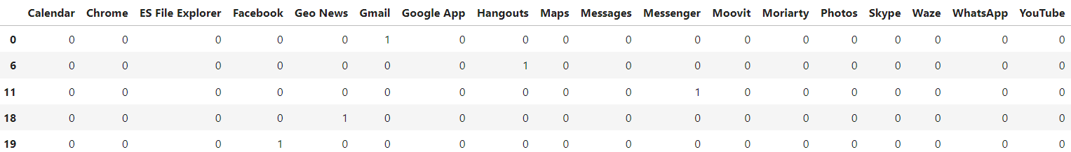
For each row, there is a single 1 corresponding to the selected category
while there is a 0 for each of the remaining columns in that row.
The table above shows the first five rows of df_labels_onehot.
Notice that there is only a single 1 in each row, with the rest being 0.
For example, the first row contains a 1 in the Maps column with the rest of
the columns containing 0.
The following two rows contain 1 in the Gmail column only.
Finally, notice that the input Series (labels)
was converted into a DataFrame.
Categorical Features Need One-Hot Encoding, Too!
Similarly, any input features that are of categorical data type must also be encoded using either integer encoding or one-hot encoding.
Which Feature Is Categorical?
There is one categorical variable among the features of the
sherlock_18appstable. Can you identify which feature is categorical? (Hint: consider thedf.head()ordf.info()output.)Solution
The
statefeature is a four-class categorical variable. This is evidenced by the data type ofstateprinted bydf.info(), ~~~ <class ‘pandas.core.frame.DataFrame’> Int64Index: 273129 entries, 0 to 999994 Data columns (total 19 columns): # Column Non-Null Count Dtype
— —— ————– —–
0 ApplicationName 273129 non-null object 1 CPU_USAGE 273077 non-null float64 2 UidRxBytes 273129 non-null int64
3 UidRxPackets 273129 non-null int64
4 UidTxBytes 273129 non-null int64
5 UidTxPackets 273129 non-null int64
6 cutime 273077 non-null float64 7 guest_time 273077 non-null float64 8 importance 273129 non-null int64
9 lru 273129 non-null int64
10 num_threads 273077 non-null float64 11 otherPrivateDirty 273129 non-null int64
12 priority 273077 non-null float64 13 rss 273077 non-null float64 14 state 273077 non-null object 15 stime 273077 non-null float64 16 utime 273077 non-null float64 17 vsize 273077 non-null float64 18 cminflt 0 non-null float64 dtypes: float64(10), int64(7), object(2) memory usage: 41.7+ MB ~~~
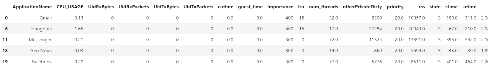
stateis the only one that has anobjectdatatype; this is the most likely candidate. All the other features have numerical in type and meaning. Take a peek at the values:df_features.head(5)
Clearly, the
statefeature is non-numerical. The number of classes in this variable can be discovered by thevalue_counts()method: ~~~python df_features[‘state’].value_counts() ~~~ ~~~python S 271951 R 995 D 114 Z 17 Name: state, dtype: int64 ~~~ Thestatefeature indicates [the state of the process]( (i.e. a running program): * S stands for “sleeping” (where the process is idle); * R indicates that the process is “running”, i.e. using much CPU; * D usually means the process is busy waiting for data from/to storage device; * Z means the process is already terminated but has not been cleaned up by the operating system.
The categorical columns in the raw table can be converted to one-hot encoding in the same way we converted the labels: ~~~python df_features = pd.get_dummies(df_features) ~~~
One-Hot Encoding in Scikit-Learn
One-hot for labels is generally not necessary in Scikit-learn. Why did we not have to explicitly apply one-hot encoding to the labels in scikit-learn? This is because ML objects such as
DecisionTreeClassifierperform this for us, behind the scene.One-hot encoding is still necessary for categorical features for Scikit-learn. Interested learners are referred to read Encoding of Categorical Variables from the Scikit-learn MOOC from INRIA for in-depth discussion.
For more information on why we need one-hot encoding, see these articles:
To summarize: With one-hot encoding, the categorical variables (including the label array, which was a vector of strings), are converted to a matrix of ones and zeros to represent input or output categorical values for NN models.
Feature Scaling
The next step we must do is to scale the features in order to normalize the values.
print("Step: Feature scaling with StandardScaler")

df_features_unscaled = df_features
scaler = preprocessing.StandardScaler()
scaler.fit(df_features_unscaled)

# Recast the features still in a dataframe form
df_features = pd.DataFrame(scaler.transform(df_features_unscaled),
                           columns=df_features_unscaled.columns,
                           index=df_features_unscaled.index)
print("After scaling:")
print(df_features.head(10))
print()
Step: Feature scaling with StandardScaler
After scaling:
    CPU_USAGE  UidRxBytes  UidRxPackets  UidTxBytes  UidTxPackets    cutime  \
0   -0.165792   -0.010623     -0.015068   -0.008245     -0.016022 -0.185461
6    0.308049   -0.010623     -0.015068   -0.008245     -0.016022 -0.185461
11  -0.140853   -0.010623     -0.015068   -0.008245     -0.016022 -0.185461
18  -0.196966   -0.010623     -0.015068   -0.008245     -0.016022 -0.185461
19  -0.143970   -0.010623     -0.015068   -0.008245     -0.016022 -0.185461
28  -0.047332   -0.003421      0.092426   -0.001260      0.149189 -0.185461
29  -0.196966   -0.010623     -0.015068   -0.008245     -0.016022 -0.185461
32  -0.200083   -0.010623     -0.015068   -0.008245     -0.016022 -0.185461
35  -0.181379   -0.010623     -0.015068   -0.008245     -0.016022 -0.185461
39  -0.206318   -0.010623     -0.015068   -0.008245     -0.016022 -0.185461

    importance       lru  num_threads  otherPrivateDirty  priority       rss  \
0     0.967513  1.621094    -0.271421          -0.188207  0.212762  0.497013
6     0.967513  1.621094    -0.830621           0.748432  0.212762  2.335413
11   -0.157189 -0.742150     1.219779          -0.039008  0.212762  1.090659
18   -0.157189 -0.742150    -0.942461          -0.555284  0.212762 -0.567867
19   -0.157189 -0.742150     1.406179          -0.312737  0.212762  0.002106
28   -0.157189 -0.742150     2.039939           0.680739  0.212762  1.858918
29    0.967513  1.621094    -0.532381          -0.336024  0.212762 -0.112617
32   -0.157189 -0.742150    -1.054301          -0.593373  0.212762 -0.918915
35    0.967513  1.305995    -0.718781          -0.435688  0.212762 -0.369580
39   -1.281891 -0.742150    -1.091581          -0.570282  0.212762 -1.120843

       stime     utime     vsize   state_D   state_R   state_S  state_Z
0  -0.335871 -0.412842  0.127145 -0.020436 -0.060473  0.064346 -0.00789
6  -0.367538 -0.431809 -0.010889 -0.020436 -0.060473  0.064346 -0.00789
11 -0.275620 -0.369463  0.487610 -0.020436 -0.060473  0.064346 -0.00789
18 -0.374264 -0.463921 -1.320928 -0.020436 -0.060473  0.064346 -0.00789
19 -0.273939 -0.384110  1.316752 -0.020436 -0.060473  0.064346 -0.00789
28 -0.108319 -0.140735  1.898536 -0.020436 -0.060473  0.064346 -0.00789
29 -0.379588 -0.463921 -1.018926 -0.020436 -0.060473  0.064346 -0.00789
32 -0.381830 -0.461104 -1.064197 -0.020436 -0.060473  0.064346 -0.00789
35 -0.352405 -0.439696 -0.751398 -0.020436 -0.060473  0.064346 -0.00789
39 -0.343438 -0.459038 -1.089401 -0.020436 -0.060473  0.064346 -0.00789
Splitting to Training and Validation Datasets
As the final step, we split the original dataset into training and validation sets (80% and 20% of the original set, respectively):
val_size = 0.2
random_state = np.random.randint(1000000)

print("Step: Train-validation split  val_size=%s  random_state=%s" \
      % (val_size, random_state))

train_features, val_features, train_L_onehot, val_L_onehot = \
    train_test_split(df_features, df_labels_onehot,
                     test_size=val_size, random_state=random_state)

print("- training dataset:   %d records" % (len(train_features),))
print("- validation dataset: %d records" % (len(val_features),))
print("Now the data is ready for machine learning!")
sys.stdout.flush()
The use and reporting of random_state argument in train_test_split
is necesssary to reproduce the computation.
Training and Validating Neural Network Models
Let us train and validate a couple of neural network models and observe how they perform to classify the various running apps.
Model with No Hidden Layers
We will begin by defining the simplest neural network model, which has no hidden layers:
model = Sequential([
    Dense(18, activation='softmax', input_shape=(19,),
          kernel_initializer='random_normal')
])
This code construct is similar to that introduced in the previous episode to create a single-neuron model. A thorough explanation of this code has been given in the previous episode, so we only recap the most important points and make mention of the additional options.
-
Only one dense layer is defined, which will be the output layer. The input layer is not presented as a separate layer here, as it literally simply passes on the input features with no modification. The output layer feeds directly from the input; there is no hidden layer. After one-hot encoding, the
sherlock_18appsinput dataset contains 19 features—thus, theinput_shape=(19,)argument. (As a reminder,(19,)refers to a tuple with one element, not a mere number 19. Do not omit the trailing comma.) There are 18 neurons in this layer, equivalent to the 18 output elements of the one-hot-encoded labels. The number of the neurons must be 18, because the model must distinguish among the 18 applications contained in the dataset. -
The
activationargument defines the type of nonlinear function used to yield the response of each neuron in this layer. Today, therelu(ReLU = Rectified Linear Unit) function is a popular choice for hidden neurons. In classification models, the output layer needs to yield the (approximately) one-hot outcome—that is, one for the target class, and zero elsewhere. Therefore, the output layer typically uses thesoftmaxorsigmoidactivation function. Thesoftmaxfunction is more widely used today. -
(Optional) The optional
kernel_initializerargument determines what kind of initial values are given to the the weights of the neurons. Therandom_normalchoice sets the values to a random values drawn from a normal distribution function (e.g. Gaussian function with unit standard deviation). This is a more advanced feature that may need to be tweaked later, as necessary. To learn more, refer to this article: A Gentle Introduction To Weight Initialization for Neural Networks. (Generally, we do not need to tweak this option at this stage of learning about NN; but such proper weight initialization will be important in real-world NN modeling since it affects the speed of convergence and/or whether the model training would converge at all.)
Please note that the model defined by a Sequential object
like that shown in the code snippet above
only declares the logical structure of the model,
but has not built it for training and deployment.
To make the model operable in Keras,
we must compile it by including the specification of
the optimizer, learning rate, loss function,
and the metrics for evaluating the model’s performance.
It is often helpful to define a function which will prepare a neural network model ready to for training, like this one for a model without hidden layer:
def NN_Model_no_hidden(learning_rate):
    """Definition of deep learning model with no hidden layer"""
    # (optional if these were already imported earlier)
    from tensorflow.keras.models import Sequential
    from tensorflow.keras.layers import Dense
    from tensorflow.keras.optimizers import Adam

    model = Sequential([
        Dense(18, activation='softmax', input_shape=(19,),
              kernel_initializer='random_normal')
    ])
    adam_opt = Adam(learning_rate=learning_rate,
                    beta_1=0.9, beta_2=0.999,
                    amsgrad=False)
    model.compile(optimizer=adam_opt,
                  loss='categorical_crossentropy',
                  metrics=['accuracy'])
    return model
In this function, a single dense layer is defined.
The Adam optimizer is created and the model is “compiled”
by combining the layer definition, optimizer, loss function.
The compiled model object is ready for training.
Training and Validation: No Hidden Layer
Let us create and train the NN model with no hidden layer. A learning rate of 0.0003 is used along with 5 epochs and a batch size of 32. In the following episode, we will run experiments and vary these parameters.
model_0 = NN_Model_no_hidden(0.0003)
history_0 = model_0.fit(train_features,
                        train_L_onehot,
                        epochs=5, batch_size=32,
                        validation_data=(val_features, val_L_onehot),
                        verbose=2)
Epoch 1/5
6827/6827 - 6s - loss: 1.6855 - accuracy: 0.5588 - val_loss: 1.2626 - val_accuracy: 0.7095
Epoch 2/5
6827/6827 - 5s - loss: 1.1122 - accuracy: 0.7378 - val_loss: 1.0053 - val_accuracy: 0.7692
Epoch 3/5
6827/6827 - 5s - loss: 0.9280 - accuracy: 0.7854 - val_loss: 0.8720 - val_accuracy: 0.7924
Epoch 4/5
6827/6827 - 5s - loss: 0.8196 - accuracy: 0.8032 - val_loss: 0.7852 - val_accuracy: 0.8079
Epoch 5/5
6827/6827 - 5s - loss: 0.7454 - accuracy: 0.8167 - val_loss: 0.7229 - val_accuracy: 0.8214
Note how the values change after each epoch and note the timing of each epoch.
Specifically, observe that the validation accuracy (val_accuracy:) starts at
around 71% and increases at a relatively constant rate until reaching 82%
once finishing the final epoch.
Analyzing Training Outcomes
When training a neural network model, we must closely watch the progression of the training by examining the values of the loss function and metrics during the training iterations. These values tell how much the model improves during these iterations, and may also indicate warnings if anything goes wrong during the training.
Let us examine more closely the history of the model training,
which is contained in the object returned by the fit function.
This object has a History data type:
print(history_0)
<keras.callbacks.History object at 0x14b0d54b3ad0>
We are interested in two important attributes of the History object,
which are history (with a lowercase “h”) and epoch:
print(history_0.history)
{'loss': [1.6854664087295532,
  1.1121711730957031,
  0.9279801845550537,
  0.8196166753768921,
  0.7453991174697876],
 'accuracy': [0.5587679147720337,
  0.7377930283546448,
  0.7854216694831848,
  0.8032326102256775,
  0.8167086839675903],
 'val_loss': [1.2626335620880127,
  1.005321979522705,
  0.8719977736473083,
  0.7851505279541016,
  0.7229281663894653],
 'val_accuracy': [0.7094624042510986,
  0.7691702246665955,
  0.7924234867095947,
  0.8078951239585876,
  0.8213893175125122]}
print(history_0.epoch)
[0, 1, 2, 3, 4]
The history attribute contains a dict (a Python key-value mapping)
with four keys, matching those printed out during the model training:
loss and accuracy computed with the training set,
and val_loss and val_accuracy computed with the validation set.
The values are the lists of the metrics computed during each epoch.
(The loss is always computed, whereas the other metrics computed
are determined by the list of metric names fed to the metrics argument
when building the model—see the compile(..., metrics=...)
function call earlier.)
Creating a History DataFrame
The
historydata structure above looks almost like a DataFrame with four columns–that is indeed true! Construct a DataFrame calleddf_history_0from this structure, and useepochattribute to populate the index.Hint
df_history_0 = pd.DataFrame(data=..., index=...)Solution
df_history_0 = pd.DataFrame(data=history_0.history, index=history_0.epoch)We will use this type of DataFrame later in this lesson.
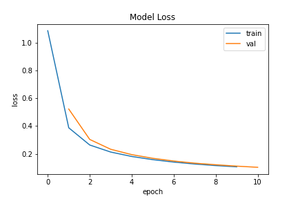
Visualizing the Training Progress
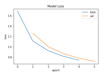
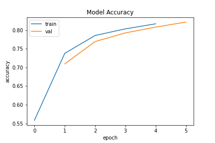
Visualization is an excellent tool to help us analyze the training progress. The training history object contains the necessary values to plot. We will introduce the following two functions to plot the loss function and the accuracy as a function of the number of epochs elapsed:
def plot_loss(model_history):
    '''Plots the values of the loss function for the training
    and validation datasets.
    '''
    epochs = np.array(model_history.epoch)
    plt.plot(epochs, model_history.history['loss'])
    plt.plot(epochs+1, model_history.history['val_loss'])
    plt.title('Model Loss')
    plt.ylabel('loss')
    plt.xlabel('epoch')
    plt.legend(['train', 'val'], loc='upper right')
    fig = plt.gcf()
    plt.show()
    return fig

def plot_acc(model_history):
    '''Plots the values of the accuracy for the training
    and validation datasets.
    '''
    epochs = np.array(model_history.epoch)
    plt.plot(epochs, model_history.history['accuracy'])
    plt.plot(epochs+1, model_history.history['val_accuracy'])
    plt.title('Model Accuracy')
    plt.ylabel('accuracy')
    plt.xlabel('epoch')
    plt.legend(['train', 'val'], loc='upper left')
    fig = plt.gcf()
    plt.show()
    return fig
Let’s call these functions now:
fig_loss0 = plot_loss(history_0)
fig_acc0 = plot_acc(history_0)
(We use the “0” suffix to denote that this is for a model
with zero hidden layer.)
Saving Training Visualization to Image Files (Optional)
The plots above can be saved as image files on disk as a visual record of the model training. Such plot image may be needed elsewhere, (e.g., for reporting to a colleague or an advisor, or for inclusion in a poster or paper):
fig_loss0.savefig("model_0H_trn0_plot_loss.png")
fig_acc0.savefig("model_0H_trn0_plot_acc.png")
We intentionally use file names that are longer to make it more descriptive:
model_0H: A model with zero hidden layer;trn0: The first training run (anticipating that more training runs may be needed);plot_accandplot_lossclearly tell which one is which plot.Feel free to devise your own naming system (including the use of directory names, which we will use in latter episodes). The crucial matter is that we must be consistent in adhering to a naming convention: This will make results easier to discover and understand, and it opens the possibility for easy automatic processing with scripts.
(Hint: When saving for publication, you may want to consider using PDF or SVG format. which yields much better quality graphics when enlarged. Simply change the filename extension from
.pngto.svg.)
Model with One Hidden Layer
Now we look at an example which builds a simple neural network model
with only hidden layer.
Our objective is to compare it with the previous no-hidden-layer model.
It is the same process as previously done,
except that another Dense layer is inserted between the input and output layer.
model = Sequential([
            Dense(hidden_neurons, input_shape=(19,), activation='relu',
                  kernel_initializer='random_normal'),
            Dense(18, activation='softmax'
                  kernel_initializer='random_normal')
        ])
Two dense layers are defined here:
The first dense layer is the hidden layer,
which feeds directly from the input data
(after various preprocessing and one-hot encoding where needed).
The second layer connects to, and takes the inputs from, the first layer.
We follow the standard practice of using relu activation function
for the hidden layer, and softmax for the output layer.
Below is a graphical depiction of the neural network model with
hidden_neurons = 24. The input layer is shown in yellow and it contains 19
neurons.
The green-colored layer in the middle is that hidden layer and the red-colored
layer is the output layer with 18 neurons.

def NN_Model_1H(hidden_neurons,learning_rate):
    """Definition of deep learning model with one dense hidden layer"""
    # (optional if these were already imported earlier)
    from tensorflow.keras.models import Sequential
    from tensorflow.keras.layers import Dense
    from tensorflow.keras.optimizers import Adam
    # define the network
    model = Sequential([
        Dense(hidden_neurons, activation='relu',
              input_shape=(19,),
              kernel_initializer='random_normal'),
        Dense(18, activation='softmax',
              kernel_initializer='random_normal')
    ])
    # define the optimization algorithm
    adam_opt = optimizers.Adam(learning_rate=learning_rate,
                               beta_1=0.9, beta_2=0.999,
                               amsgrad=False)
    model.compile(optimizer=adam_opt,
                  loss='categorical_crossentropy',
                  metrics=['accuracy'])
    return model
This function takes two parameters:
hidden_neurons, specifying the number of the neurons in the hidden layer;learning_rate, determining the step size at each iteration.
Training and Validation: Model with One Hidden Neuron
Now, let’s create an actual model (saving it to a Python variable named model_1)
and train it:
model_1 = NN_Model_1H(18, 0.0003)
model_1.summary()
history_1 = model_1.fit(train_features,
                        train_L_onehot,
                        epochs=10, batch_size=32,
                        validation_data=(val_features, val_L_onehot),
                        verbose=2)
Model Hyperparameters
Please note the hyperparameters used in this model.
Solution
We use
hidden_neurons= 18,learning_rate= 0.0003, andbatch_size= 32 as our baseline.
Calling the summary method will provide a tabular summary of the model:
Model: "sequential_1"
_________________________________________________________________
Layer (type)                 Output Shape              Param #
=================================================================
dense_1 (Dense)              (None, 18)                360
_________________________________________________________________
dense_2 (Dense)              (None, 18)                342
=================================================================
Total params: 702
Trainable params: 702
Non-trainable params: 0
This provides a helpful description of the model’s architecture.
The first layer, named dense_1, is the hidden layer.
The second layer, dense_2, is the output layer.
(The names were assigned automatically by Keras;
they can be overriden by specifying name= argument
when declaring the Dense layer object.)
Here’s an example of the training output:
Epoch 1/10
6827/6827 - 7s - loss: 1.0861 - accuracy: 0.6885 - val_loss: 0.5226 - val_accuracy: 0.8783
Epoch 2/10
6827/6827 - 6s - loss: 0.3877 - accuracy: 0.9080 - val_loss: 0.3039 - val_accuracy: 0.9289
Epoch 3/10
6827/6827 - 6s - loss: 0.2638 - accuracy: 0.9393 - val_loss: 0.2331 - val_accuracy: 0.9477
Epoch 4/10
6827/6827 - 6s - loss: 0.2131 - accuracy: 0.9508 - val_loss: 0.1946 - val_accuracy: 0.9552
Epoch 5/10
6827/6827 - 6s - loss: 0.1814 - accuracy: 0.9582 - val_loss: 0.1683 - val_accuracy: 0.9592
Epoch 6/10
6827/6827 - 6s - loss: 0.1585 - accuracy: 0.9638 - val_loss: 0.1485 - val_accuracy: 0.9657
Epoch 7/10
6827/6827 - 6s - loss: 0.1410 - accuracy: 0.9683 - val_loss: 0.1332 - val_accuracy: 0.9695
Epoch 8/10
6827/6827 - 6s - loss: 0.1270 - accuracy: 0.9719 - val_loss: 0.1218 - val_accuracy: 0.9717
Epoch 9/10
6827/6827 - 6s - loss: 0.1159 - accuracy: 0.9743 - val_loss: 0.1118 - val_accuracy: 0.9755
Epoch 10/10
6827/6827 - 6s - loss: 0.1069 - accuracy: 0.9765 - val_loss: 0.1034 - val_accuracy: 0.9755
This training process above has 10 epochs.
At the end of each epoch, the total time taken to complete epoch is printed
(about 7 seconds),
the value of the loss function (loss:) is printed, and the
accuracy (accuracy:) of the prediction.
(Accuracy here refers to the fraction of training data outcomes that
are correctly categorized by the network at that particular instance
in time.)
As we see, the accuracy increases as we take more epochs.
Finally, the val_accuracy is computed using the
validation data which we set aside earlier for this purpose.
Your accuracy and loss numbers would not be identical to that printed above,
but should be close, because the initial weights of the network would not
be identical from run to run due to random initialization.
We get a pretty good accuracy using this model only after 5 epochs, but it still is a few percentage points from 100%.
Plotting Training Progress
Following the procedure previously done, make two plots (one for loss vs epoch, the other for accuracy vs epoch), to visually inspect how the model’s performance improves as a result of the training. (Hint: we saved the output of
model_1.fit()to a variable namedhistory_1.)Discuss the following questions with your fellow learners (if available):
Quantify the improvement in accuracy at the end of epoch 5 compared to the previous model (
model_0– the model without any hidden layer, versusmodel_1with one hidden layer).If we had trained with more epochs, what could be the accuracy at larger epoch values? What would be the upper limit of the model’s accuracy? (Answer/discuss these questions for both
model_0andmodel_1.)Solution
fig_loss_1 = plot_loss(history_1)
fig_acc_1 = plot_acc(history_1)
» Potential discussion responses:
- At epoch 5, the model with no hidden layer (
model_0)
Limit of Accuracy
What will be the ultimate accuracy of the network defined in
model_1above, if we can train longer?
Saving and Loading a Neural Network Model
Model training is computationally very expensive;
a trained model is therefore a valuable asset to preserve.
At the end of a successful model training,
we will want to save the model to disk (a permanent storage medium)
for later uses.
In Keras, this can be done using the save method:
model_1.save("model_1_e10.h5")
The _e10 suffix in the filename reminds us that this model was trained
with 10 epochs from the initially random weights.
This procedure will save the important properties of model_1:
The architecture (e.g. the number of layers;
the type, size, and activation function of each layer),
the hyperparameters (learning rate, optimizer, etc.),
the model’s parameters (weights and biases),
and many more.
A Keras model saved in this way can be reloaded and used
either in this Python session or in a completely different program.
To load a saved model, use the load_model function:
from tensorflow.keras.models import load_model
model_1_reload = load_model("model_1_e10.h5")
Check the reloaded model’s architecture – it must return the same structure as the original model:
model_1_reload.summary()
Model: "sequential_1"
_________________________________________________________________
Layer (type)                 Output Shape              Param #
=================================================================
dense_1 (Dense)              (None, 18)                360
_________________________________________________________________
dense_2 (Dense)              (None, 18)                342
=================================================================
Total params: 702
Trainable params: 702
Non-trainable params: 0
_________________________________________________________________
Inference
Inference refers to the act of using a machine learning model to make predictions. Tnference takes the input data in the same format as the feature matrix (or a single record) used in the training: In other words, the input data must pass through the same postprocessing stages. The difference is that only forward propagation takes place; there is no more learning or weight adjustment taking place.
Let’s take a single sample from the sherlock_18apps table:
sample0 = train_features.iloc[[0], :]
print(sample0)
        CPU_USAGE  UidRxBytes  UidRxPackets  UidTxBytes  UidTxPackets  \
908302  -0.047332   -0.010623     -0.015068   -0.008245     -0.016022

          cutime  importance       lru  num_threads  otherPrivateDirty  \
908302 -0.185461    0.967513  1.621094    -0.644221          -0.378258

        priority      rss     stime     utime     vsize   state_D   state_R  \
908302  0.212762  0.56176 -0.368098 -0.449649 -0.512512 -0.020436 -0.060473

         state_S  state_Z
908302  0.064346 -0.00789
The truth label is given by:
label0 = train_L_onehot.iloc[0]
print(label0)
Calendar            0
Chrome              0
ES File Explorer    0
Facebook            0
Geo News            0
Gmail               0
Google App          0
Hangouts            0
Maps                1
Messages            0
Messenger           0
Moovit              0
Moriarty            0
Photos              0
Skype               0
Waze                0
WhatsApp            0
YouTube             0
Name: 908302, dtype: uint8
If expressed in terms of the index of the label that is “hot”, it will be:
print(label0.argmax())
8
So, what’s the prediction of the model?
The inference is done by calling the model’s predict() method:
pred0 = model_1_reload.predict(sample0)
print(pred0)
[[2.4963332e-02 6.7778787e-04 1.1179425e-01 1.6566955e-06 4.0571130e-14
  2.0663649e-02 6.1197621e-05 1.2832742e-06 8.4175241e-01 4.0272408e-09
  7.4097048e-23 4.1409818e-12 1.1227924e-07 3.3482531e-05 5.0862218e-05
  3.4804633e-09 1.6152820e-23 1.4111901e-11]]
We can take the original model (model_1)
or the reloaded model as shown in the example above;
the result must be the same.
What is this? It is a 1x18 matrix which indicates the predicted label in the one-hot format. Index of the element with the highest value will be the predicted label:
print(pred0.argmax())
8
Great! Our model made a correct answer for this one input.
Batch Inference
Inference can also take an array of samples instead of a single sample. Repeat the procedure above but using multiple samples. Take the first 10 samples from the training data and perform an inference, and compare against the ground-truth labels.
samples_b1 = val_features.head(10)
print(samples_b1)
CPU_USAGE UidRxBytes UidRxPackets UidTxBytes UidTxPackets \ 225731 -0.200083 -0.010623 -0.015068 -0.008245 -0.016022 729777 -0.115914 -0.010623 -0.015068 -0.008245 -0.016022 957188 -0.200083 -0.010623 -0.015068 -0.008245 -0.016022 865739 -0.196966 -0.010623 -0.015068 -0.008245 -0.016022 904012 -0.078506 -0.010623 -0.015068 -0.008245 -0.016022 810264 -0.200083 -0.010623 -0.015068 -0.008245 -0.016022 568396 7.443720 0.873325 1.382347 0.248574 1.925208 253495 -0.187614 -0.010623 -0.015068 -0.008245 -0.016022 755631 -0.053567 -0.010623 -0.015068 -0.008245 -0.016022 864667 -0.147088 -0.010623 -0.015068 -0.008245 -0.016022 cutime importance lru num_threads otherPrivateDirty \ 225731 -0.185461 -0.157189 -0.742150 -0.756061 -0.469632 729777 -0.185461 0.967513 0.360697 -0.905181 0.534303 957188 -0.185461 -0.157189 -0.742150 -0.681501 -0.587255 865739 -0.185461 0.967513 1.621094 -0.942461 -0.448516 904012 -0.185461 0.967513 1.621094 -0.830621 0.878093 810264 -0.185461 -0.157189 -0.742150 -1.054301 -0.597517 568396 -0.185461 0.967513 0.990895 -0.159581 0.115323 253495 -0.185461 -0.157189 -0.742150 1.406179 -0.337406 755631 0.379995 -0.157189 -0.742150 0.735139 0.776456 864667 -0.185461 0.967513 1.621094 -0.308701 -0.224322 priority rss stime utime vsize state_D state_R \ 225731 0.212762 -0.593765 -0.332789 -0.431997 -1.241426 -0.020436 -0.060473 729777 0.212762 -0.547633 0.018348 -0.111252 -0.450473 -0.020436 -0.060473 957188 0.212762 -1.001062 -0.334190 -0.314628 -0.614857 -0.020436 -0.060473 865739 0.212762 -0.466902 -0.379028 -0.469179 -0.686304 -0.020436 -0.060473 904012 0.212762 2.511039 -0.373703 -0.444579 0.193941 -0.020436 -0.060473 810264 0.212762 -0.551073 -0.383231 -0.461480 -1.064197 -0.020436 -0.060473 568396 0.212762 2.535319 -0.374264 -0.444015 -0.363264 -0.020436 -0.060473 253495 0.212762 -0.034516 -0.194071 -0.289464 0.653661 -0.020436 -0.060473 755631 0.212762 1.265070 0.701004 0.867133 0.334266 -0.020436 -0.060473 864667 0.212762 0.540515 -0.347081 -0.414532 -0.090737 -0.020436 -0.060473 state_S state_Z 225731 0.064346 -0.00789 729777 0.064346 -0.00789 957188 0.064346 -0.00789 865739 0.064346 -0.00789 904012 0.064346 -0.00789 810264 0.064346 -0.00789 568396 0.064346 -0.00789 253495 0.064346 -0.00789 755631 0.064346 -0.00789 864667 0.064346 -0.00789Here are the ground-truth labels:
labels_b1_onehot = val_L_onehot.head(10)
print(labels_b1_onehot)
Calendar Chrome ES File Explorer Facebook Geo News Gmail \ 225731 0 0 0 0 1 0 729777 0 1 0 0 0 0 957188 0 0 0 0 0 0 865739 0 0 0 0 0 0 904012 0 0 0 0 0 0 810264 0 0 0 0 0 0 568396 0 0 0 0 0 0 253495 0 0 0 0 0 0 755631 0 0 0 0 0 0 864667 0 0 0 0 0 1 Google App Hangouts Maps Messages Messenger Moovit Moriarty \ 225731 0 0 0 0 0 0 0 729777 0 0 0 0 0 0 0 957188 0 0 0 0 0 1 0 865739 0 0 0 0 0 0 0 904012 0 1 0 0 0 0 0 810264 0 0 0 0 0 0 0 568396 0 0 0 0 0 0 0 253495 0 0 0 0 1 0 0 755631 0 0 0 0 0 0 0 864667 0 0 0 0 0 0 0 Photos Skype Waze WhatsApp YouTube 225731 0 0 0 0 0 729777 0 0 0 0 0 957188 0 0 0 0 0 865739 0 0 1 0 0 904012 0 0 0 0 0 810264 1 0 0 0 0 568396 0 1 0 0 0 253495 0 0 0 0 0 755631 0 0 0 1 0 864667 0 0 0 0 0Solution
Here are the model’s predictions:
preds_b1_onehot = model_1_reload.predict(samples_b1)
print(preds_b1_onehot.shape)
with np.printoptions(precision=3, suppress=True, linewidth=150):
    print(preds_b1_onehot)
(10, 18) [[0. 0. 0. 0. 1. 0. 0. 0. 0. 0. 0. 0. 0. 0. 0. 0. 0. 0. ] [0. 1. 0. 0. 0. 0. 0. 0. 0. 0. 0. 0. 0. 0. 0. 0. 0. 0. ] [0. 0. 0. 0. 0. 0. 0.012 0. 0. 0. 0. 0.984 0. 0.004 0. 0. 0. 0. ] [0. 0.038 0.024 0. 0. 0. 0. 0. 0. 0. 0. 0. 0. 0.001 0. 0.936 0. 0. ] [0. 0. 0. 0. 0. 0.002 0. 0.998 0. 0. 0. 0. 0. 0. 0. 0. 0. 0. ] [0. 0. 0. 0. 0.034 0. 0.003 0. 0. 0. 0. 0. 0. 0.962 0. 0. 0. 0. ] [0. 0.002 0.491 0. 0. 0.025 0. 0.03 0.106 0.062 0. 0. 0. 0.192 0.09 0. 0. 0. ] [0. 0. 0. 0.001 0. 0. 0. 0. 0. 0. 0.998 0. 0. 0. 0. 0. 0. 0. ] [0. 0. 0. 0. 0. 0. 0. 0. 0. 0. 0. 0. 0. 0. 0. 0. 1. 0. ] [0.06 0. 0.014 0. 0. 0.922 0. 0. 0.002 0. 0. 0. 0. 0. 0.002 0. 0. 0. ]]The predicted labels (by integer indices):
preds_b1 = preds_b1_onehot.argmax(axis=1)
print(preds_b1)
[ 4 1 11 15 7 13 2 10 16 5]The ground-truth labels is a little tricky because we must get to the underlying array to do so; but here’s the formula:
labels_b1 = labels_b1_onehot.values.argmax(axis=1)
print(labels_b1)
[ 4 1 11 15 7 13 14 10 16 5]Finally, here’s the verification of predicted labels against the ground truths:
print(np.equal(preds_b1, labels_b1))[ True True True True True True False True True True]It’s not bad to have 90% correct answer; this should not be all that typical given the high accuracy of the model (97%). Statistically, more than 95% prediction should be correct.
Make the following evaluation:
- Compare the accuracy of this model at the different epoch numbers (e.g. 10, 20, 30).
- If we train further, what could be the accuracy at large epoch values?
- How much improvement do we have by epoch 10 from the previous model without any hidden layer?
Traditional Machine Learning
Now, we will compare our Deep Learning models to the traditional machine learning algorithms learned
in the previous session.
Here we test on Decision Tree and Logistic Regression.
To simplify the code, we will use the model_evaluate function to evaluate the performance of a machine
learning model (whether traditional ML or neural network model).
def model_evaluate(model,test_F,test_L):
    test_L_pred = model.predict(test_F)
    print("Evaluation by using model:",type(model).__name__)
    print("accuracy_score:",accuracy_score(test_L, test_L_pred))
    print("confusion_matrix:","\n",confusion_matrix(test_L, test_L_pred))
    return
Decision Tree
ML_dtc = DecisionTreeClassifier(criterion='entropy',
                                   max_depth=6,
                                   min_samples_split=8)
%time ML_dtc.fit(train_features, train_labels)
CPU times: user 897 ms, sys: 8.37 ms, total: 906 ms
Wall time: 906 ms

DecisionTreeClassifier(ccp_alpha=0.0, class_weight=None, criterion='entropy',
                       max_depth=6, max_features=None, max_leaf_nodes=None,
                       min_impurity_decrease=0.0, min_impurity_split=None,
                       min_samples_leaf=1, min_samples_split=8,
                       min_weight_fraction_leaf=0.0, presort='deprecated',
                       random_state=None, splitter='best')
model_evaluate(ML_dtc, test_features, test_labels)
Evaluation by using model: DecisionTreeClassifier
accuracy_score: 0.9497216932766954
confusion_matrix:
 [[ 1829     1     0     0     0     0     0     0     0     0     0    18     0     0     0     0     1     0]
 [    0  5477     0     0     0    69     0     0     0     0     0     0     0     5     0     0     2     0]
 [    1   610  2753     0     0    25     0     5     0     1     1     1     0     2     0     0     0     0]
 [    0     0     0  4029     0     0    15     0     0     0     0     0     0     0     0     0     0    10]
 [    0     0     0     0  4006     0     0     0     0     0     0     0     0     0     0     0     0     0]
 [   64    28     0     0     0  3183     1     0     0     0     0     1     0    49     0     0     0     0]
 [    0   143     0     0     0     2 10459     0     0     0    15     0     0     0     0     0  1369     0]
 [    0    58     0     0     0    24     4  1408     0     1     0     0     0     1     0     0    11     0]
 [    3    39     0     0     0     0     1     0   935     0     0     0     0     0     1     0     4     0]
 [    0     0     0     0     0     0     0     0     1   486     0     0     0     8     0     0     0     0]
 [    0     0     0     0     0     0     0     0     0     0  4016     0     0     0     0     0     0     0]
 [    0     0     0     0     0     0     0     0     0     0     0  1697     0     0     0     0     0     0]
 [    0    13     0     0     4     0     0     0     0     0     0     0   680     1     0     0     0     0]
 [    0     0     0     0     0     0     0     0     0     0     0     6     0  3473     0     0     0     0]
 [    0     0     0     0     0     0     0     0     0     0     0     0     0     0  1003     0     0     0]
 [    0     0     0     0     3     0     0     0     0     0     0     0     0     0     0  1642     0     0]
 [    0     4     0     0     0     0     4     0     0     0     0     0     0     0     0     0  3897     0]
 [    0     0     0     0     0   116     0     0     0     0     0     0     0     0     0     0     0   897]]
Logistic Regression
ML_log = LogisticRegression(solver='lbfgs')
%time ML_log.fit(train_features, train_labels)
CPU times: user 20.6 s, sys: 2.48 s, total: 23 s
Wall time: 23.1 s

/shared/apps/auto/py-scikit-learn/0.22.2.post1-gcc-7.3.0-wpia/lib/python3.7/site-packages/sklearn/linear_model/_logistic.py:940: ConvergenceWarning: lbfgs failed to converge (status=1):
STOP: TOTAL NO. of ITERATIONS REACHED LIMIT.

Increase the number of iterations (max_iter) or scale the data as shown in:
    https://scikit-learn.org/stable/modules/preprocessing.html
Please also refer to the documentation for alternative solver options:
    https://scikit-learn.org/stable/modules/linear_model.html#logistic-regression
  extra_warning_msg=_LOGISTIC_SOLVER_CONVERGENCE_MSG)

LogisticRegression(C=1.0, class_weight=None, dual=False, fit_intercept=True,
                   intercept_scaling=1, l1_ratio=None, max_iter=100,
                   multi_class='auto', n_jobs=None, penalty='l2',
                   random_state=None, solver='lbfgs', tol=0.0001, verbose=0,
                   warm_start=False)
model_evaluate(ML_log, test_features, test_labels)
Evaluation by using model: LogisticRegression
accuracy_score: 0.9197854108686099
confusion_matrix:
 [[ 1387     3    63     0     0   319     0     0     0     0     0     0     0    72     5     0     0     0]
 [    0  4590   390     0     0    37    77    10     6    64     0     0     0    72    31   273     3     0]
 [   60   271  2817     0     0     7    13     4     0     0     0     0     0    85   141     1     0     0]
 [    0     1     0  4021     0     2    11     4     0     0     5     0     0     0     0     2     0     8]
 [    0     0     0     0  3999     0     0     0     0     7     0     0     0     0     0     0     0     0]
 [   47    39    14     0     0  3189    24    10     1     0     0     0     0     2     0     0     0     0]
 [    7    93     0    51     0    19 11628     8     0     0    29    58     0     0     0     0    93     2]
 [    0    28     0     2     0    33     1  1442     0     0     0     1     0     0     0     0     0     0]
 [  147    27   673     0     0     1     0     0   113     0     0     0     0     4     7     0    11     0]
 [    0     0     0     0     0     0     0     0     0   433     0     0     0    24     0    38     0     0]
 [    0     0     0     0     0     0     0     0     0     0  4016     0     0     0     0     0     0     0]
 [    0     0     0     0     0     0     3     0     0     0     0  1642     0    52     0     0     0     0]
 [    0     1     0     0     0     0     0     1     0     4     0     0   692     0     0     0     0     0]
 [   17     2   239     0     0     0     0     0    17    31     0     0     0  3080    80    13     0     0]
 [   99     5   172     0     0    45     0     0     7     0     0     0     0     2   673     0     0     0]
 [    0     3     0     2     0     0     0     0     0     0     0     0     0     6     0  1634     0     0]
 [    0     0     0     0     0     0    33     0     0     0     0     0     0     0     0     0  3872     0]
 [    0     0     0     0     0     0     0     0     0     0     0     0     0     0     6     0     0  1007]]
By now, we have a pretty good background knowledge about this dataset, and we know the accuracy scores we can get by using the Decision Tree and Logistic Regression methods, which are reasonably good, but a few percentage points away from 99%. Our Decision Tree model ended up performing with nearly identical accuracy to our Neural Network with one hidden layer, which means we need to find ways to create models with higher accuracy in order for it to make sense to use Neural Networks. We will explore these ways later.
Further improvement
Except we can tune those two hyper-parameters, there are a lot of things we can do
in Neural Network. For example:
1. Using activation function sigmoid instead of relu
2. Using 1000 epochs instead of 10 epochs
3. Adding more hidden layers
4. Using different optimizer algorithmns.
Overall, the trend of the train and dev loss and accuracy should be monitored and relevant hyperparameters should be modified based on the results.
Key Points
On KERAS, we can easily build the network by defining the layers and connecting them together.