An Introduction to Keras with Binary Classification Task
Overview
Teaching: 0 min
Exercises: 0 minQuestions
What is Keras?
What are the advantages of using Keras to build neural network models?
What are the basic steps for building a neural network model in Keras?
Objectives
Understanding Keras and its relationship to other neural network libraries available in the community.
Understanding the steps required to build, train, and validate basic neural network models in Keras.
Introduction
Keras is a high-level software framework for building, training, and deploying neural network (NN) models. Keras provides a high-level interface to another framework named TensorFlow, which implements the actual complex mathematical algorithms for NN training and inference. Keras offers an easy-to-use application programming interface (API) in the Python programming language. As we shall see shortly, expressing an NN model using Keras is quite intuitive. Keras allows the user to focus on the structure of the network model without having to be concerned with low-level mathematical details.
In this episode, we will use Keras and
the preprocessed sherlock_2apps dataset
to build and train a simple NN model for a binary classification task,
i.e. distinguishing two smartphone apps.
This is an extremely simple model for such a powerful ML method,
but with it we shall learn all the fundamentals of
building, training, and validating an NN model.
This fundamental knowledge and skillset will be applicable to
all realistic and most complicated NN models.
Defining a Neural Network in Keras
Required Python Libraries
First, let us import the necessary Python libraries and classes:
import os
import sys
import pandas as pd
import numpy as np
from matplotlib import pyplot as plt
import sklearn

# Borrow data preparation and model validation tools from scikit-learn:
from sklearn import preprocessing
from sklearn.model_selection import train_test_split
from sklearn.metrics import accuracy_score, confusion_matrix
# Classic machine learning models:
from sklearn.linear_model import LogisticRegression
from sklearn.tree import DecisionTreeClassifier

# TensorFlow & Keras
import tensorflow as tf
import tensorflow.keras as keras

# Import Keras objects
from tensorflow.keras.models import Sequential
from tensorflow.keras.layers import Dense
from tensorflow.keras.optimizers import Adam
The Keras API is accessed via the tensorflow.keras Python module.
Since Keras is quite a complex library, it is subdivided into
many submodules.
There are three basic Keras submodules that we should know:
-
tensorflow.keras.layerscontains the various layer classes that can be used to build NN models.Denserepresents the fully connected neuron layer, the most basic form of NN layers. -
tensorflow.keras.modelscontains the model-focused classes and functions, including theSequentialandModelobjects (representing the sequential and functional models, respectively, as explained below), model training functions, and model saving/loading functions. -
tensorflow.keras.optimizerscontains the various optimizer algorithms, used to adjust the weights (and/or bias) of the Keras NN model (based on loss).
(Many more submodules are available.)
These three submodules are interrelated and represent the three basic building blocks of a NN model in Keras: A Keras model consists of one or more layers that are arranged in a specific order. An optimizer defines an algorithm that adjusts the parameters during the training process.
Data Preparation
Let us load and prepare the
sherlock_2appsdata (features and labels) to train a classification NN model. The data is already preprocessed and only need to be split into training and validation datasets usingtrain_test_split, provided by scikit-learn:df2_features = pd.read_csv('sherlock/2apps_4f/sherlock_2apps_features.csv') df2_labels = pd.read_csv('sherlock/2apps_4f/sherlock_2apps_labels.csv') train_F, val_F, train_L, val_L = train_test_split(df2_features, df2_labels, test_size=0.2)In the split above, 80% of the data are used for training and 20% for validating (testing) the model.
Neuron, Layer, Network: Constructing a Model
There are two main ways we can programmatically build models in Keras, corresponding to two different APIs: sequential model API and functional model API.
Sequential Model API
A sequential model creates models layer-by-layer, with the outputs of the previous layer connecting to the inputs of the subsequent layer. This easy-to-use API is useful to construct a straightforward NN model that has exactly one input data and one output data. (A single input could be a multi-dimensional array of values; similarly for the output.)
Limitations of sequential models:
-
They cannot create multiple models that share layers.
-
They cannot create models where layers have multiple inputs and outputs.
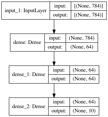
Figure: An example of a sequential NN model, visualized by the Keras API. This network may be trained to perform digit recognition by using the MNIST dataset (having 28 x 28 pixel input data and 10-category output data). Source: Keras Developer’s Guide.
Functional Model API
The functional model provides a way to create arbitrarily complicated models that include layer sharing, multiple inputs or outputs (to the model), requires any layers with multiple inputs and/or outputs, or a non-linear topology (such as a multi-branch model). In this lesson, we will focus on the sequential model. Once we understand how to build a network with the sequential model, it will be straightforward to learn the functional model. Jason Brownlee shows how models can be constructed using the functional model API.
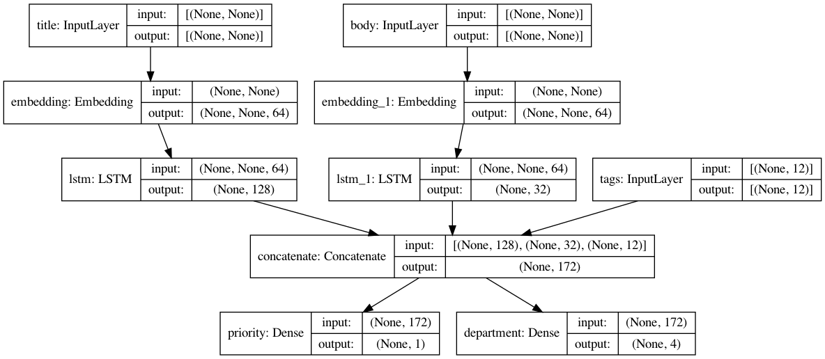
Figure: An example of a complex functional model from the Keras API. Source: Keras Developer’s Guide.
Examples of Complex Neural Network Models
The model depicted in the figure above could be useful for analyzing text-based documents or emails. The model has three distinct inputs (title, text body, and tags) and returns two output values (the priority and the appropriate department for the document). The three inputs are fed together into one network, and the network is trained to classify both the appropriate priority and department of the documents it analyzes. Other complex networks that need the functional API include models with feedback loops. These complex models are beyond the scope of this introductory lesson.
Defining a Neuron Layer
Let us create a single Dense layer, with only one neuron,
that takes in four input features and outputs one number
(0 or 1, to indicate the app described by the input features):
dense1 = Dense(1, activation='sigmoid', input_shape=(4,))
A Dense layer creates a standard, fully-connected neuron layer,
which can be a visible (input or output) or a hidden layer.
The Dense arguments have the following meaning:
-
1(orunits=1) indicates the number of output values from this layer, which also defines the number of fully-connected neurons. -
activation='sigmoid'defines the (nonlinear) activation function used to transform the weighted sum of the input values to the output values. -
input_shape=(4,)indicates that this layer is connected to an input layer that has four inputs. Theinput_shapeargument can be defined only on the first layer directly connected to the input layer. (Please note that the value must be given as a tuple, not a single number. The comma after the number 4 is not optional.)
Please refer to Keras’ documentation for the Dense layer for more information and additional parameters.
Defining a Neural Network Model
Keras’ Sequential object defines an NN model that takes the form
of a simple sequence of layers.
The layers can be declared at the same time that the Sequential model is constructed,
as follows:
model = Sequential([
            Dense(1, activation='sigmoid', input_shape=(4,))
        ])
In this example, there is only one layer, which is the output layer.
Now, we can print a useful summary of the model by using model.summary().
This will print a table with the folowing columns:
-
Name and type of all the layers in the model as layer_name (layer type).
-
Output shape (i.e. dimensionality) for each layer, as a list or tuple.
-
Number of weight parameters of each layer.
It also includes the following information listed under the table:
- The total number of parameters as well as the number of trainable parameters and non-trainable parameters.
Note that null or None in the output shape represents that the number is
flexible and depends on the batch size of the inputs.
model.summary()
Model: "sequential"
_________________________________________________________________
Layer (type)                 Output Shape              Param #
=================================================================
dense (Dense)                (None, 1)                 5
=================================================================
Total params: 5
Trainable params: 5
Non-trainable params: 0
_________________________________________________________________
Where Are the Parameters?
Each
Denselayer contains weights that will be optimized while training the network. Each neuron (within theDenselayer) has a bias parameter that can also be optimized. Parameters are internal variables and refer to both weights and bias. For a fully-connected layer that has \(N\) neurons connected to \(M\) input values, there will be \(N * (M + 1)\) weights, where the extra factor 1 comes from the bias. As a consequence, a deep neural network with many layers will quickly accummulate an enormous number of weights, especially if the fully-connected layers have many neurons.For the example above, there are four inputs \(M = 4\) and 1 neuron \(N = 1\). So, there are 5 parameters/weights.
How Many Parameters Are There?
How many adjustable parameters are in the following NN model?
Figure: A NN model with one hidden layer. (Image modified from Glosser.ca.)
Solution
The network consists of 3 input values, a layer with 4 hidden neurons, and 2 output values. The hidden layer consists of 4 neurons \(M = 4\) with 3 inputs \(N = 3\) (from the input layer); so there are 16 parameters.
The outer layer consists of 2 neurons \(M = 2\) with 4 inputs \(N = 4\), so 10 more parameters.\(4 * (3+1) + 2 * (4+1) = 26.\) In total, there are 26 parameters.

Preparation for Training
In order to train the NN model we defined above, we need a few additional components:
-
Loss function: quantifies the error of the network’s predictions when compared to the ground-truth labels in the training or validation data. The goal of the training phase is to minimize the loss function, i.e. to make the model predict the expected outcomes as accurately as possible.
-
Optimization algorithm: a predefined algorithm used to iteratively improve the model during the training phase. This will be explained further in this section.
-
Learning rate: a tuning hyperparameter in the optimization algorithm that determines the “step size” at each iteration while moving toward a minimum of the loss function.
How an Optimization Algorithm Works in Training a Neural Network Model
Training an NN model involves progressively updating the weights and bias of the neurons through backpropagation until the errors made by the model’s prediction are sufficiently minimized. These errors are quantified by a loss function, sometimes also called a cost function. Training a neural network model is as much of an art as it is a science. The use of an appropriate optimization algorithm is critical for ensuring that we obtain the best model.
When a new model is trained for the first time, the weights are typically initialized to random values. Among the various methods for optimizing NN models, gradient descent has become a general method of choice, optimizing an NN model by minimizing its error function. The following graphics illustrate how gradient descent works:
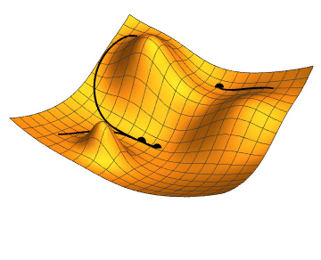
Figure: An illustration of gradient descent for two-parameter (weights and bias) optimization. Three optimization scenarios are indicated by the three black points and their tracks. Two points converge to the same terminal endpoint, but one converges to a different endpoint. The linked Wikimedia source includes animated graphics that demonstrate the progression of the optimization algorithm. Source: Jacopo Bertolotti, Wikimedia.
Imagine a single-neuron model that has only two weight parameters (e.g. two weights and no adjustable bias). The loss function, plotted as a function of these parameters, will look like the mountainous terrain shown in the picture above. The x and y-axes are the weights and the z-axis is the loss. The model will start with a set of parameters, represented as a tiny “dot” on this terrain. The slope (negative gradient) of the terrain plus the imaginary “downward gravity” will pull this “dot” along a certain trajectory until it meets the lowest point of a valley (i.e. lowest loss value). Gradient descent is an iterative algorithm by which the “dot” is moved through successive steps until the lowest point is closely reached. In machine learning terms, Gradient Descent is an iterative algorithm by which the parameters are updated to minimize the loss. This, in a nutshell, is how the gradient descent algorithm works!
However, as the same illustration shows, not all the “dots” or initializations of the parameters reach the same final point, as the parameters could get stuck in a higher valley, often called a local minimum. For this reason, it is often necessary to repeat the training process by starting with different initial parameter values. Another way is to provide a different step amount to provide more confidence regarding the optimality of the trained model.
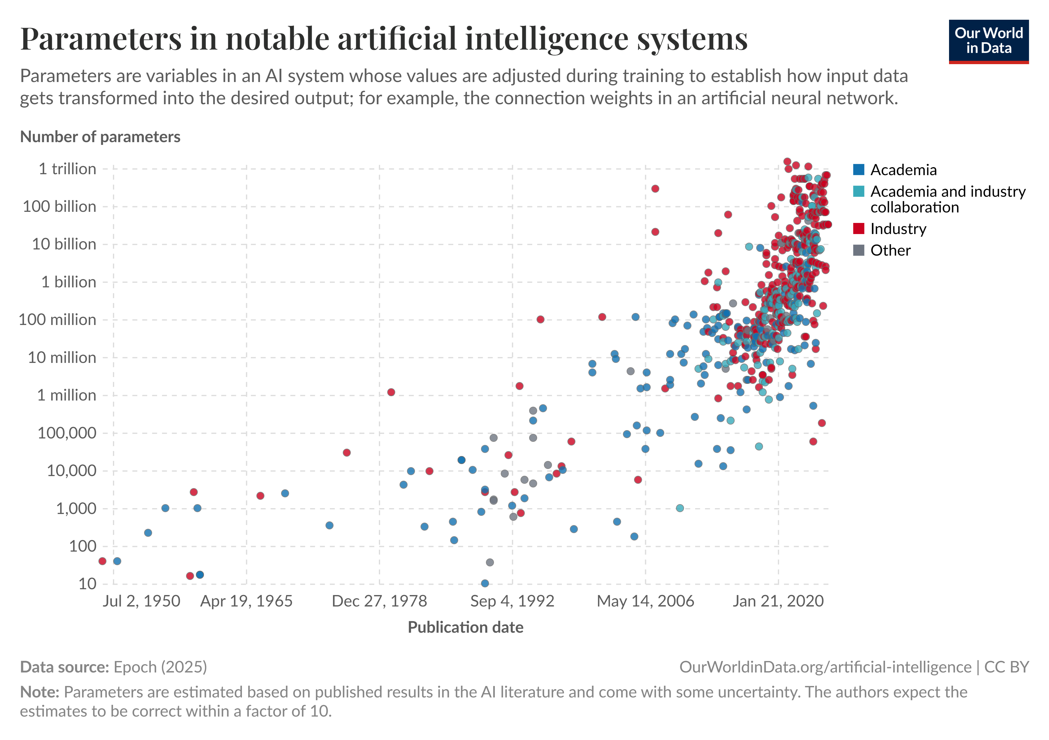
In an actual network optimization scenario, the gradient descent algorithm must work in a high-dimensional space, according to the number of adjustable parameters in the network model. This can involve many millions, or even billions, of parameters. For example, the AlexNet model, which set the record for image classification accuracy in 2012, has over 62 million parameters. More recently, a powerful text-generation NN model called GPT-3, introduced in 2021, has over 175 billion parameters! According to Our Data World, some algorithms have more than 1 trillion parameters! The sheer dimensionality of the parameter space alone indicates that it can be very challenging to train an NN model correctly and optimally. There are many tricks to help reduce the amount of time needed to train a model. For example, weights saved from a previously trained model can often be used as the initial values to speed up the training.
Figure: A graphical representation of the number of parameters in notable AI systems.
A detailed discussion on NN optimization algorithms is beyond the scope of this short training program. Some examples can be found in the reference section of this lesson and at ruder.io.
Defining an Optimizer
Let us now create an optimizer,
which encapsulates the optimization algorithm used to improve the network
during the training process.
The tensorflow.keras.optimizers module contains many algorithms
that can be used to train the network.
Each algorithm has its own strengths and weaknesses
that make it suitable for certain types of use cases.
We will be using the Adam optimizer, which was designed to effectively optimize neural networks in a wide range of scenarios:
adam_opt = Adam(learning_rate=0.0003, beta_1=0.9, beta_2=0.999, amsgrad=False)
Adam is a specific variant of the gradient descent algorithm implementation and has recently seen broad adoption in many application areas, such as computer vision and natural language processing. An article by Jason Brownlee, Gentle Introduction to the Adam Optimization Algorithm for Deep Learning, provides a gentle introduction to the Adam optimizer. Interested readers can also learn more about this optimizer in a paper, “Adam: A Method for Stochastic Optimization”, written by Diederik P. Kingma and Jimmy Ba, the original inventors of this algorithm.
The learning rate (explained below) must be determined
when the optimizer object is created.
The Adam optimizer will automatically adjust the learning rate
as the training progresses.
The rate of this adjustment is determined by two hyperparameters:
β1 and β2.
The following optional arguments to Adam object creation can
tweak the optimizer’s behavior:
beta_1: An exponential decay rate for the first moment estimates.beta_2: An exponential decay rate for the second moment estimates.epsilon: A small constant needed for the algorithm’s numerical stability.amsgrad: A boolean variable that controls whether to apply the AMSGrad variant of the optimizer. AMSGrad is a further refinement of Adam that is supposed to improve its convergence in some challenging cases.
Please consult Keras API for Adam optimizer for more information about the Keras API for the Adam optimizer.
Learning Rate
The learning rate is a most important hyperparameter that controls how much the model parameters (neuron weights and/or biases) are changed according to the corrections estimated by backpropagation. The learning rate must be a real number between 0 and 1: 0 means that the model is not changed at all (i.e. ignoring changes estimated by backpropagation), whereas 1 means that an aggressive correction based on the backpropagation results is necessary. Typically, we use a value that is very small (closer to 0). For example, Keras’ default value for the learning rate is 0.001; we will start with a smaller value, which means a more conservative model update.
In choosing an appropriate learning rate, there is a trade-off between the rate of convergence (how fast the weights are changed from one iteration to the other) and the stability (whether the algorithm is making its way toward the lowest minimum of the loss function) of the algorithm. Additionally, a learning rate that is too small may lead to a suboptimal model because the parameters may become stuck in a local minimum. We must therefore find a “sweet spot” to obtain the most optimal model within a reasonable amount of time. For a more detailed explanation, see this article: Understand the Impact of Learning Rate on Neural Network Performance. We will revisit the issue of learning rate in a later lesson.
Loss Function
The loss function determines how the error in the NN model’s prediction is quantified. Just like the optimizers, many kinds of loss functions are used in real applications, each tailored for a specific kind of machine learning task. There are two important functions that we must know when working with classification tasks:
-
Binary cross-entropy loss, designed for binary classification tasks such as the ML task at hand with the
sherlock_2appsdataset. -
Categorical cross-entropy loss, for multi-class classification tasks (i.e. classification involving more than two categories).
These loss functions are provided by Keras under the
tensorflow.keras.losses submodule.
In Keras, the choice of the loss function is specified when we compile the NN model
(see the loss argument of the compile function in the next section).
The various loss functions provided by the Keras package can be found in
Keras API documentation on Losses.
The most frequently used loss functions and their specific
applications are described briefly in this article:
“Understanding Different Loss Functions for Neural Networks”.
Compiling the Model: Putting Them All Together
As a final step before training the model in Keras, we need to compile the model.
The compile function of the model object ties three components together:
the neural model itself,
the optimizer,
and the loss function.
This step furnishes a workable model that can be trained and later used for inference.
Here is the code:
model.compile(optimizer=adam_opt,
              loss='binary_crossentropy',
              metrics=['accuracy'])
The key compile arguments are:
optimizer: The optimizer algorithm. We useadam_opt, the Adam optimizer object already created earlier.loss: The loss function. See below for more details.metrics: The list of performance metrics to be evaluated and reported at the end of each epoch. The main metric we will use in this lesson is accuracy, although precision and recall may need to be considered for certain applications (e.g. malware detection).
For the loss function specification,
Keras allows us to specify the function name as a string (as we did above)
or the constructed object (i.e. tf.keras.losses.BinaryCrossentropy()).
It also allows for the creation of custom metrics.
The loss functions for classification problems can be specified in this way:
-
For binary classification tasks:
loss='binary_crossentropy'orloss=tf.keras.losses.BinaryCrossentropy(). -
For multi-class classification tasks:
loss='categorical_crossentropy'orloss=tf.keras.losses.CategoricalCrossentropy().
Congratulations, now the model is truly ready for training! Let us now train the model and observe how well it performs.
Recap: Steps in Neural Network Model Construction
Based on the discussion and hands-on code you have learned so far, please recap the steps required to construct an NN model in Keras using the model sequential API.
Solution
Step 1: Define the NN model by creating the
Sequentialobject and declaring the layers of the network in its argument.model = Sequential([ Dense(1, activation='sigmoid', input_shape=(4,)) ])Step 2: Create an optimizer object to be used in the training phase. This includes defining the learning rate value.
adam_opt = Adam(learning_rate=0.0003, beta_1=0.9, beta_2=0.999, amsgrad=False)Step 3: Compile the model. This step will integrate the optimizer defined in step 2, the loss function, and the metric(s) for model evaluation.
model.compile(optimizer=adam_opt,
              loss='binary_crossentropy',
              metrics=['accuracy'])
Training and Validating the Model
The Keras NN model is trained by calling the fit function
of the model object:
model_history = model.fit(train_F, train_L,
                          epochs=5, batch_size=32,
                          validation_data=(val_F, val_L),
                          verbose=2)
The key arguments to fit are as follows:
train_Fandtrain_L(the first two arguments): The features and labels, respectively, from the training dataset.epochs: The number of times (i.e. iterations) that the learning algorithm will work through the dataset.batch_size: The number of samples from the training dataset to be processed at once (“as a single batch”) to compute the corrections to the network’s parameters.validation_data: Dataset (features and labels) used to validate the model’s performance metrics. This validation is performed at the end of each epoch. This must be a 2-tuple containing the feature matrix (val_F) and label matrix (val_L), respectively. Obviously, this dataset must not overlap with the training dataset.verbose: the verbosity mode. This affects how much of the training per epoch information is printed.
More on Training Algorithm: Epoch and Batch Size
Training a network is an iterative process. In each step, the optimization algorithm will perform a full sweep over the entire training dataset (called an epoch, step, or iteration), wherein the network weights are updated through the forward and backward propagation steps. In normal cases, as more iterations are performed, the loss will eventually decrease to a minimum value, in which case the optimizer has reached its goal. We therefore must supply an adequate number of
epochsin order to adequately train a network model.Another important argument to the
fitfunction is thebatch_size. Many algorithms that are used in practice perform the network weight updates in small batches (the so-called “mini-batch gradient descent”). This approach was empirically found to offer the best trade-off between computational cost and algorithm accuracy. A larger batch size results in a more accurate gradient estimate at the cost of very expensive computation. The size of the batch is an important hyperparameter that must be carefully controlled in the training phase, since it can affect the quality (e.g. accuracy) of the trained model.
Training Results
Here is an example of the results of the training,
printed by the fit function:
Epoch 1/5
15303/15303 - 38s - loss: 0.4681 - accuracy: 0.7984 - val_loss: 0.3646 - val_accuracy: 0.8491
Epoch 2/5
15303/15303 - 23s - loss: 0.3554 - accuracy: 0.8491 - val_loss: 0.3526 - val_accuracy: 0.8491
Epoch 3/5
15303/15303 - 26s - loss: 0.3497 - accuracy: 0.8491 - val_loss: 0.3500 - val_accuracy: 0.8492
Epoch 4/5
15303/15303 - 26s - loss: 0.3480 - accuracy: 0.8494 - val_loss: 0.3490 - val_accuracy: 0.8495
Epoch 5/5
15303/15303 - 25s - loss: 0.3472 - accuracy: 0.8497 - val_loss: 0.3484 - val_accuracy: 0.8496
Keras prints out a progress report at the end of every epoch
(this behavior is determined by the verbose=2 argument to the fit function).
Consider the first record printed, where the meaning of each reported field is as follows:
15303/15303– The number of training sample batches processed (in this case, 15,303 batches).38s– The amount of time taken to complete this epoch (38 seconds).loss: 0.4681 - accuracy: 0.7984– The loss and accuracy of the NN model computed using the training data. This loss function is what is being minimized during the training.val_loss: 0.3646 - val_accuracy: 0.8491– The loss function and accuracy of the NN model computed using the validation data. These metrics provide less unbiased estimates of the performance of the model.
The fit function’s output shows the results of training for 5 iterations or epochs.
In each epoch, the training algorithm goes through the all training data once
(through the forward and backward propagation passes),
then adjusts the model parameters (neuron weights and/or biases)
toward minimizing the loss
(i.e., aggregated errors in the predicted labels with respect to the training set).
As the result shows, each epoch took more than 20 seconds to complete
(this timing will vary based on the actual computer hardware used to run this training process).
Note how the loss and accuracy values change after each epoch.
Under normal conditions, the loss would decrease with increasing epoch.
At the end of five epochs, the loss drops down to just below \~0.35, and the accuracy is at \~0.85.
Interestingly, Keras by default validates the model at the end of every epoch;
therefore, we do not need to perform a separate validation.
Some Caveats
Your exact printout of the metrics will be different from the printout above, since there are variabilities and randomness associated with the NN training process (different computers, whether a GPU is used or not, and different random numbers being used). As long as the results of the same epoch number fluctuate around similar values, these results are all valid.
Keras computes the metrics from the training data before the model’s weights are updated but the metrics from the validation data after the weights are updated. As a result, the validation metrics appear to be better than the training-data metrics, but that is not the case. This difference will become negligible as the model is further refined with more epochs. As with any machine learning method in general, it is better to consider only the validation metrics to judge the performance of the trained network, because validation data provide an unbiased estimate of the model’s performance.
Recording Training History
The
fitfunction returns a data structure that contains the history of the optimization. These include the values of the loss function, measured performance metrics (such as accuracy), using training and validation data, etc. We will learn how to use this to create training plots in the next episode.
Did We Train Enough?
Consider the values of the
val_accuracymetric in the training output above. Do you think we have trained the model reasonably well? What will happen if we train the network with more epochs?Solution
Optimal model training involves a trade-off between how much computing we are willing to perform (which translates to how long we have to wait until we get the best model) and the accuracy of the model. There is also an issue of overfitting vs. underfitting. In the example above, improvement in the accuracy can only be seen in the fourth digit; hence, it is negligible. Therefore, five epochs is sufficient in this example. However, note that this is a special “toy problem”, and most real-world problems will require many more epochs.
How Did Our Model Perform?
The final accuracy of this model, according to the output printed above,
is about 85% (the last val_accuracy value).
The final loss function is just below 0.35, which did not drop much from
the first value of 0.36.
Considering that our model had only one neuron layer,
which also serves as the output layer, this is actually not bad,
though it is far from being a reliable model.
Therefore, we should expect a meager accuracy outcome.
The purpose of neural network modeling is to improve its performance
by adding as many layers as possible to achieve the best result,
within the bounds of what is computationally feasible.
Comparing Neural Network vs Traditional Machine Learning Models
We just finished constructing and testing our first NN model with Keras. It is instructive that we compare the performance results of our one-neuron model against the performance of traditional ML models.
Results from Traditional Machine Learning Methods
In the Machine Learning lesson, we introduced and studied in detail two ML models: the logistic regression and decision tree classifiers. Train these models and evaluate their accuracy scores. Please compare the accuracy of the NN model we just trained above with that of these two classic ML models.
Hint: For comparison purposes, it is helpful to define a function to evaluate a classic ML model’s performance (accuracy and confusion matrix):
def model_evaluate(model,test_F,test_L):
    test_L_pred = model.predict(test_F)
    print("Evaluation by using model:",type(model).__name__)
    print("accuracy_score:",accuracy_score(test_L, test_L_pred))
    print("confusion_matrix:\n",confusion_matrix(test_L, test_L_pred))
    return
Decision Tree
Example code & output:
model_dtc = DecisionTreeClassifier(criterion='entropy', max_depth=3, min_samples_split=8)
model_dtc.fit(train_F, train_L)
model_evaluate(model_dtc, val_F, val_L)
Evaluation by using model: DecisionTreeClassifier accuracy_score: 0.9896506375435988 confusion_matrix: [[75592 228] [ 1039 45564]]Logistic Regression
Example code & output:
model_lr = LogisticRegression(solver='lbfgs')
model_lr.fit(train_F, train_L.to_numpy().ravel())
model_evaluate(model_lr, val_F, val_L)
Evaluation by using model: LogisticRegression accuracy_score: 0.8495789189939799 confusion_matrix: [[73706 1973] [16442 30302]]Which ML model performs the best? Do you suspect that the one-neuron NN model is equal to one of these traditional models in terms of performance? What is your basis for making that claim?
Solution
As it currently stands, the best performing ML model we’ve encountered so far is actually the decision tree classifier, at around 99% accuracy! This means that the decision tree’s model architecture is flexible enough to capture the complexity in the data. In contrast, both logistic regression and the one-neuron NN have an accuracy that is about 85%, which is not very high.
Interestingly, a one-neuron NN model with a sigmoid activation function is mathematically identical to the logistic regression function. (Some minute differences exist in the training process, maybe due to the different training algorithms and different regularization terms used; however, these should not cause a qualitative difference.) This is why they have the same accuracy score. In fact, logistic regression can be thought of as the original building block of the NN model, before more variations in the activation functions and types of layers were introduced.
Programming Exercise: Encapsulating the Neural Network Model Construction
In computer programming, writing functions is an important way to help us repeat a sequence of commands efficiently. A function is essentially a callable computer subprogram that may accept user-specified parameters to vary the actions of the subprogram’s behavior.
Back to our NN modeling, it is very convenient to define a function to construct a ready-to-train NN model since we will use this many times in our experiments. As we shall see going forward, deep learning involves tedious trial-and-error runs. We will have to repeatedly modify, train, and validate our network models in order to find the most optimal one.
As an exercise, let’s create a function to construct a one-neuron model that is ready to be trained to perform the binary classification task on the
sherlock_2appsdata. It must have four inputs and one output. Here’s the skeleton:def NN_binary_clf(learning_rate): """Constructs a one-neuron binary classifier using Keras.""" model = ... ... return modelAfter this function, one should be able to simply construct and train the Keras model in this way:
# An example invocation:
model1 = NN_binary_clf(0.0003)
history1 = model1.fit(...)
Question 1: First, remind yourself: What are the required steps to include in the
NN_binary_clffunction above?Solution 1
- Define the NN model
- Define the optimizer
- Compile the NN model to bring together the optimizer, loss function, and model evaluation metrics.
Question 2: Now, write the contents (definition) of the
NN_binary_clffunction. Use the same choices as we used earlier for the optimizer, loss function, etc.Solution 2
def NN_binary_clf(learning_rate):
    """Create a one-neuron binary classifier using Keras.
    `learning_rate` is the only adjustable hyperparameter here."""
    from tensorflow.keras.models import Sequential
    from tensorflow.keras.layers import Dense
    from tensorflow.keras.optimizers import Adam
    model = Sequential([
                Dense(1, activation='sigmoid', input_shape=(4,))
            ])
    adam_opt = Adam(learning_rate=learning_rate,
                    beta_1=0.9, beta_2=0.999, amsgrad=False)
    model.compile(optimizer=adam_opt,
                  loss='binary_crossentropy',
                  metrics=['accuracy'])
    return model
Note: The importation of Keras objects (
Sequential, etc.) is optional, but this will allow the function to be used anywhere regardless of the availability of these objects as global symbols.
Improving the Neural Network Model
Discuss with your colleague: What can we do to improve our one-neuron NN model? What will be the simplest next step? If possible, implement the improvement by creating and training a new model. What is the accuracy of the new model?
Solution
The easiest next step is to add one hidden layer. As a starting example, this hidden layer can have five neurons. The training and validating of this model is left for learners to do on their own as a very simple exercise. One may ask, what about having only three or two neurons in this layer? Which version will be the best?
Summary
In this episode, we learned the basic mechanics of building and training a neural network model using Keras. We used a binary classification task to distinguish between only two apps: Facebook and WhatsApp. While this is a rather basic problem, we have learned a lot of important concepts that we must know to carry out deep learning modeling.
Spoiler: Performance Summary Notes for
sherlock_2appsClassificationIn terms of performance, the trained one-neuron model above had an accuracy score (
val_acc) of around 85%. Compared to the results of classic ML methods in the Machine Learning lesson, this NN performance was the same as that of logistic regression, significantly below the \~99% achievable with the decision tree model.By adding more layers, the NN method can afford us extremely flexible models that can easily outperform any traditional ML technique. In later episodes, we will learn how to achieve better results with neural networks by adding more hidden neurons. We will also discuss when one ought to use deep learning approaches and when traditional ML methods should be used instead.
Steps of Deep Learning with Keras
- Import necessary libraries (TensorFlow, scikit-learn);
- Load the clean, preprocessed datasets (labels and features);
- Split the data into training and testing datasets;
- Design the neural network model architecture (i.e. what types of layers to use, how many neurons per layer, and which activation function to choose);
- Declare the neural network model using either a sequential or functional API;
- Select an optimizer and determine its hyperparameters;
- Select a loss function;
- Compile the model;
- Fit the model using training data, and validate with validation data.
Key Points
Keras is an easy-to-use high-level API for building neural networks.
Main parts of a neural network layer: number of hidden neurons, activation function.
Main parts of a neural network model: layers, optimizer, learning rate, loss function, performance metrics.