Tuning Neural Network Models for Better Accuracy
Overview
Teaching: 15 min
Exercises: 50 minQuestions
What is model tuning in Deep Learning?
What are the different types of tuning applicable to a neural network model?
What are the effects of tuning a particular hyperparameter to the performance of a model?
Is Jupyter notebook the best platform for such experiments?
Objectives
Tweak and tune deep learning models to obtain optimal performance.
Describe the common hyperparameters that can be varied to tune a neural network model.
Understand the steps of post-processing and the set-up required for post-analysis.
Introduction
In the previous episode, we successfully built and trained a few neural network (NN) models to distinguish 18 running apps in an Android phone. We tested a model without hidden layer, as well as a model with one hidden layer. We saw a significant improvement of accuracy by adding just one hidden layer. This poses an interesting question: What is the limit of NN models in achieving the highest accuracy (or a similar performance metric)? We can intuitively expect that increasing the complexity of the model might result in better and better accuracy. One way we explored this (in the previous episode) was by increasing the number of hidden layers. We can continue this refinement by constructing models with two, three, four hidden layers, and so on and so forth. The number of combinations will explode quickly, as each layer may also be varied in the number of hidden neurons. Every modified model must be retrained, which will make the entire process prohibitively expensive. We inevitably would have to stop the refinement at a certain point. All these experimentations constitute model tuning, an iterative process of refining an NN model by adjusting hyperparameters to yield better results for the given task (such as smartphone app classification, in our case).
In this episode, we will present a typical scenario for tuning an NN model. Consider the case of 18-apps classification task again: All the models have 19 input and 18 output nodes. The hidden layers of the model can be greatly varied, for example:
- A model with no hidden layer
- A model with one hidden layer of 18 neurons
- A model with two hidden layers of 18 neurons each
- A model with two hidden layers of 36 and 18 neurons, respectively
- … and many more!
What Are the Hyperparameters to Adjust?
The following hyperparameters in a model can be adjusted to find the best-performing NN model:
- the number of hidden layers (i.e. the depth of the network)
- the number of neurons for each hidden layer (i.e. the width of the layer)
Collectively, the size of network inputs and outputs, plus the number of hidden layers and the number of neurons on each hidden layer, determine the architecture of an NN model.
The learning rate (step size) and batch size (the number of training samples before updating) can also be adjusted. Although they are not part of the network architecture per se, they may affect the final accuracy of the model. So it is also important to find the optimal values for these hyperparameters as well.
Basic Procedure of Neural Network Model Tuning
The tuning process involves scanning the hyperparameter space, re-training the newly modified network and evaluate the model performance. A basic recipe for NN model tuning involves the following steps:
-
First, define the hyperparameter space we want to scan (e.g. the number of hidden layers = 1, 2, 3, …; the number of hidden neurons = 25, 50, 75, …).
-
Define (build) a new NN model with a specified hyperparameter setting (number of hidden layers, number of neurons in each layer, learning rate, batch size, …).
-
Train and evaluate the new model. From this process, we will want to compute and save the performance metrics of this model (i.e., one or more of: accuracy, precision, recall, etc.).
-
Repeat steps 1 and 2 until all the configurations we want to test have been tested. As you may anticipate, we will have to do a lot of trainings (at least one training per model).
-
Once we obtain all the performance metrics from each model, we will analyze these results to decide the most optimal NN model hyperparameter setting to achieve the best performance.
The following diagram shows the cycle of NN model tuning:
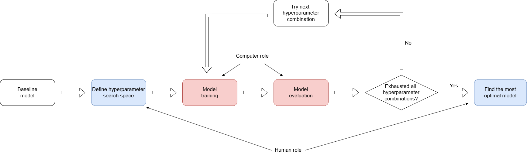
Figure: This diagram shows the cycle of NN model tuning.
The optimal configuration is determined by the trade-off of the maximally achieveable performance metrics (such as accuracy), versus the computational cost of training even more complex NN models.
Python Library: Gathering Useful Tools into a Toolbox
Instructor’s Notes
In this section, we guide learners into standard software engineering practices such as modularity (dividing a computer program into separate, independent, and self-contained units called modules) and reusability (defining functions to embody frequently used steps/procedures in multiple programs). As an introductory training, this lesson aims to provide basic exposure to these practices by guiding them through practical, step-by-step demonstrations. An instructor may treat this section as optional (for example, due to the shortage of time, or if their learners are more experienced in proramming). Instead, one can provide an overview of
sherlock_ML_toolbox.pyat the end of this section and move onto the next section–the meat of model tuning.
Before diving into the model tuning experiments,
it will be beneficial to gather useful functions into a toolbox.
This toolbox will be called my_toolbox.py.
This toolbox will include much of the code from
the previous episode on NN modeling for the sherlock_18apps dataset,
in a cleaner and more organized fashion.
Use the provided my_toolbox.py as a starting place.
From this point, we will program in Python more intensively
as we need to repeat many computations that are very similar (or identical)
in nature.
Preparing Python Environment & the Dataset
Let us prepare our Python environment in the same way as in previous episode,
then load and preprocess the sherlock_18apps data.
Loading Libraries
First, load the Python libraries.
"""
The starting toolbox for the sherlock_18apps dataset.
"""

import sys

import pandas as pd
import numpy as np

from sklearn import preprocessing
from sklearn.model_selection import train_test_split

import matplotlib.pyplot as plt

# tools for deep learning:
import tensorflow as tf
import tensorflow.keras as keras

# Import key Keras objects
from tensorflow.keras.models import Sequential
from tensorflow.keras.layers import Dense
from tensorflow.keras.optimizers import Adam

# CUSTOMIZATIONS (optional)
np.set_printoptions(linewidth=1000)
Loading in and Preprocessing the Data
Programming Challenge: Writing a Function for Data Preprocessing,
load_prep_data_18apps().Now, let’s create a
load_prep_data_18apps()function. This function will load the sherlock_18apps dataset and do the preprocessing for ML and NN modeling: data cleaning, label/feature separation, feature normalization/scaling, etc. until it is ready for ML except for train-validation splitting. It will return a 5-element tuple.def def load_prep_data_18apps(): """ToDo: Load in the sherlock_18apps dataset""" """ToDo: Summarize the dataset""" """ToDo: Clean the dataset: Delete irrelevant features and missing or bad data""" """ToDo: Separate labels from features""" """ToDo: Perform one-hot encoding for **all** categorical features.""" """ToDo: Feature scaling using StandardScaler.""" return \ df, \ # (DataFrame) the original raw data df2, \ # (DataFrame) the cleaned data labels, \ # (Series) the cleaned labels, original format df_labels_onehot, \ # (DataFrame) the cleaned labels, one-hot encoded df_features # (DataFrame) the cleaned features, preprocessed for MLPlease refer to “Data Preprocessing and Cleaning: A Review” section on the previous episode for the content and the expected outcome.
Step 1: Load in the sherlock_18apps dataset.
To do: Load in the sherlock_18apps dataset. Hint: use read_csv().
Solution
datafile = "sherlock/sherlock_18apps.csv"
print("Loading input data from: %s" % (datafile,))
df = pd.read_csv(datafile, index_col=0)
Step 2: Summarize the dataset.
To do: summarize the dataset. Hint: use
shape,info(), anddescribe().T.Solution
print("* shape:", df.shape)
print()
print("* info::\n")
print(df.info())
print()
print("* describe::\n")
print(df.describe().T)
print()
Step 3: Clean the dataset.
To do: Perform cleaning on the Sherlock 19F17C dataset. All the obviously bad and missing data are removed. Hint: utilize
df.drop().Solution
# Missing data or bad data
del_features_bad = [
    'cminflt', # all-missing feature
    'guest_time', # all-flat feature
]
df2 = df.drop(del_features_bad, axis=1)

print("Cleaning:")
print("- dropped", len(del_features_bad), "columns: ", del_features_bad)

print("- remaining missing data (per feature):")
isna_counts = df2.isna().sum()
print(isna_counts[isna_counts > 0])

print("- dropping the rest of missing data")
df2.dropna(inplace=True)

print("- remaining shape: %s" % (df2.shape,))
Step 4: Separate labels from the features.
To do: Separate labels from the features. Hint: The labels are the application name and the features is everything else but the label. Utilize
df2.drop()again.Solution
print("Step: Separating the labels (ApplicationName) from the features.")
labels = df2['ApplicationName']
df_features = df2.drop('ApplicationName', axis=1)
Step 5: Perform one-hot encoding.
To do: Perform one-hot encoding: for all categorical features. Hint: utilize
pd.get_dummies().Solution
df_labels_onehot = pd.get_dummies(labels)

print("Step: Converting all non-numerical features to one-hot encoding.")
df_features = pd.get_dummies(df_features)
Step 6: Feature scaling using
StandardScaler.To do: Feature scaling using
StandardScaler. Hint: fit theStandardScalar.Solution
print("Step: Feature scaling with StandardScaler")

df_features_unscaled = df_features
scaler = preprocessing.StandardScaler()
scaler.fit(df_features_unscaled)

# Recast the features still in a dataframe form
df_features = pd.DataFrame(scaler.transform(df_features_unscaled),
                          columns=df_features_unscaled.columns,
                          index=df_features_unscaled.index)
print("After scaling:")
print(df_features.head(10))
print()
return \
    df, \
    df2, \
    labels, \
    df_labels_onehot, \
    df_features
To test the function, create a new script that imports
my_toolbox.py, run the function, and then print out the return values. They should match the output from the previous episode.
Splitting the Dataset
Programming Challenge: Writing a Function for Splitting the Dataset,
split_data_18apps().Now, let’s create a
split_data_18apps()function. This function performs data splitting (train-test split) into training and validation dataset. It will return a 6-element tuple.def split_data_18apps(df_features, labels, df_labels_onehot): """Performs data splitting (train-test split) into training and validation datasets. Args: df_features (DataFrame): The (cleaned & scaled) feature matrix. labels (Series): The cleaned labels, original format. df_labels_onehot (DataFrame): The cleaned labels, one-hot encoded. Returns: A 6-element tuple containing the following: ( train_features, # (DataFrame) training set, feature matrix val_features, # (DataFrame) validation set, feature matrix train_labels, # (Series) training set, labels in original format val_labels, # (Series) validation set, labels in original format train_L_onehot, # (DataFrame) training set, labels in one-hot encoding val_L_onehot # (DataFrame) validation set, labels in one-hot encoding ) """ return \ train_features, val_features, \ train_labels, val_labels, \ train_L_onehot, val_L_onehotPlease refer to “Splitting to Training and Validation Datasets” section on the previous episode for the content and the expected outcome. Similar to above, use the provided
my_toolbox.pyas a starting point for the function.Splitting the dataset.
Hint: Utilize
train_test_split.Solution
def split_data_18apps(df_features,
                      labels,
                      df_labels_onehot):
    val_size = 0.2

    #random_state = np.random.randint(1000000)
    random_state = 34

    print("Step: Train-validation split  val_size=%s  random_state=%s" \
          % (val_size, random_state))

    train_features, val_features, train_labels, val_labels = \
       train_test_split(df_features, labels,
                        test_size=val_size, random_state=random_state)

    print("- training dataset:   %d records" % (len(train_features),))
    print("- validation dataset: %d records" % (len(val_features),))
    print("Now the data is ready for machine learning!")
    sys.stdout.flush()

    # Post-split the one-hot reps of the labels (classes) here,
    # which are needed for neural networks modeling.
    train_L_onehot = df_labels_onehot.loc[train_labels.index]
    val_L_onehot = df_labels_onehot.loc[val_labels.index]

    print("Now the dataset is ready for machine learning!")
    return \
        train_features, val_features, \
        train_labels, val_labels, \
        train_L_onehot, val_L_onehot
To test the function, create a new script that imports
my_toolbox.py, run the function, and then print out the return values. They should match the output from the previous episode.
Creating the NN_Model_1H Function
Programming Challenge: Writing a Function for Creating the Model,
NN_Model_1H()Now, let’s create a
NN_Model_1H()function. This function defines and compiles a deep learning model with one dense hidden layer. It will return a sequential NN model.def NN_Model_1H(hidden_neurons, learning_rate): """Defines and compiles a deep learning model with one dense hidden layer. Args: hidden_neurons (int): The number of neurons in the first (hidden) Dense layer. learning rate (float > 0): The learning rate for the Adam optimizer. Returns: The Sequential NN model created. """ return modelPlease refer to “Model with One Hidden Layer” section on the previous episode for the content and the expected outcome. Similar to above, use the provided
my_toolbox.pyas a starting point for the function.Creating the Sequential Model, Create the Adam Optimizer, and Print Model Information.
Hint: This will be similar to the Sequential models already created, but with the hidden neurons passed in as a variable
hidden_neurons. Remember to create the Adam optimizer.Solution
def NN_Model_1H(hidden_neurons, learning_rate):
    random_normal_init = tf.random_normal_initializer(mean=0.0, stddev=0.05)
    model = Sequential([
        # More hidden layers can be added here
        Dense(hidden_neurons, activation='relu', input_shape=(19,),
              kernel_initializer=random_normal_init), # Hidden Layer
        Dense(18, activation='softmax',
              kernel_initializer=random_normal_init)  # Output Layer
    ])
    adam_opt = Adam(learning_rate=learning_rate, beta_1=0.9, beta_2=0.999, amsgrad=False)
    model.compile(optimizer=adam_opt,
                  loss='categorical_crossentropy',
                  metrics=['accuracy'])

    print("Created model: NN_Model_1H")
    print(" - hidden_layers  = 1")
    print(" - hidden_neurons = {}".format(hidden_neurons))
    print(" - optimizer      = Adam")
    print(" - learning_rate  = {}".format(learning_rate))
    print()

    return model
To test the function, create a new script that imports
my_toolbox.py, run the function, and then print out the return values. They should match the output from the previous episode.
Creating Plotting Functions
Programming Challenge: Writing a Function for Plotting the Loss,
plot_loss().Now, let’s create a
plot_lossfunction. This function plots the training and validation loss over epochs.def plot_loss(model_history): """ Plot the progression of loss function during an NN model training, given the model's history. Loss computed with both the training and validation datasets during the training process are plotted in one graph. Hint: Utilize the plt.plot() function for both the loss and val_loss. Args: model_history (History): The History object returned from NN model training function, Model.fit(). """Please refer to the “Visualizing the Training Progress” section on the previous episode for the content and the expected outcome. Similar to above, use the provided
my_toolbox.pyas a starting point for the function.Create the
plot_loss()function.Hint: Utilize the plt.plot() function for both the loss and val_loss.
Solution
def plot_loss(model_history):
    epochs = model_history.epoch
    plt.plot(epochs, model_history.history['loss'])
    plt.plot(epochs, model_history.history['val_loss'])
    plt.title('Model Loss')
    plt.ylabel('loss')
    plt.xlabel('epoch')
    plt.legend(['train', 'val'], loc='upper right')
    plt.show()
To test the function, create a new script that imports
my_toolbox.py, run the function, and then print out the return values. They should match the output from the previous episode.
Programming Challenge: Writing a Function for Plotting the Accuracy,
plot_acc().Now, let’s create a
plot_accfunction. This function plots the training and validation accuracy over epochs.def plot_acc(model_history): """ Plot the progression of accuracy during an NN model training, given the model's history. Accuracy computed with the training and validation datasets during the training process are plotted in one graph. Hint: Utilize the plt.plot() function for both the accuracy and val_accuracy. Args: model_history (History): The History object returned from NN model training function, Model.fit(). """Please refer to the “Visualizing the Training Progress” section on the previous episode for the content and the expected outcome. Similar to above, use the provided
my_toolbox.pyas a starting point for the function.Create the
plot_acc()function.Hint: Utilize the plt.plot() function for both the accuracy and val_accuracy.
Solution
def plot_acc(model_history):
    epochs = model_history.epoch
    plt.plot(epochs, model_history.history['accuracy'])
    plt.plot(epochs, model_history.history['val_accuracy'])
    plt.title('Model Accuracy')
    plt.ylabel('accuracy')
    plt.xlabel('epoch')
    plt.legend(['train', 'val'], loc='upper right')
    plt.show()
To test the function, create a new script called
my_toolbox_tester.ipynbthat importsmy_toolbox.py, runs the functions, and then print out the return values. They should match the output from the previous episode.
sherlock_ML_toolbox: Toolbox for Machine Learning Modeling with SherLock Dataset
We have developed a toolbox–a Python module–called sherlock_ML_toolbox,
to simplify the Python codes that train and validate sherlock_18app
classification models.
Here are a brief description of some key functions in sherlock_ML_toolbox:
-
load_prep_data_18appsandsplit_data_18appsfunctions collectively perform the data preparation steps before the model training, including data loading, cleaning, preprocessing all the way to train-validation data split. -
NN_Model_1Hbuilds the neural network model with one hidden layer for thesherlock_18appclassification. -
plot_loss,plot_acc,combine_loss_acc_plotsfunctions provide ways to visually inspect the training progress in terms of loss and/or accuracy. -
The rest of the functions (such as
fn_dir_tuning_1H,fn_out_history_1H,fn_dir_tuning_XH,fn_out_history_XH, …) provide systematic organization for the model tuning results. These functions will be explained later.
The sherlock_ML_toolbox module contains all functions that were written
earlier for your own my_toolbox;
the key difference is that the functions in sherlock_ML_toolbox are further improved
to allow more flexibility for the users of the toolbox.
For example, sherlock_ML_toolbox.load_prep_data_18apps
has a parameter named datafile that allow the user to specify the datafile path.
To learn more about this function, use the help function in Jupyter
or Python interpreter to print the function’s documentation:
import sherlock_ML_toolbox
help(sherlock_ML_toolbox.load_prep_data_18apps)
Help on function load_prep_data_18apps in module sherlock_ML_toolbox:

load_prep_data_18apps(datafile, print_summary=True)
    Loads the sherlock_18apps dataset and do the preprocessing for
    ML and NN modeling: data cleaning, label/feature separation,
    feature normalization/scaling, etc. until it is ready for ML
    except for train-validation splitting.

    Args:
      datafile: The pathname of the data file. This must be a CSV file.
        The conventional file name is "sherlock/sherlock_18apps.csv".
      print_summary (optional): A switch to print info about the dataset or
        some summary or excerpt of the data.

    Returns:
      A 5-element tuple containing the following:

      (
        df,                  # (DataFrame) the original raw data
        df2,                 # (DataFrame) the cleaned data
        labels,              # (Series) the cleaned labels, original format
        df_labels_onehot,    # (DataFrame) the cleaned labels, one-hot encoded
        df_features          # (DataFrame) the cleaned features, preprocessed for ML
      )
The sherlock_ML_toolbox module contains a powerful plotting function
called combine_loss_acc_plots,
which display the loss and accuracy plots side-by-side
from a given model’s history.
The remaining functions in the sherlock_ML_toolbox.py file are helper functions
to create directory and file names,
which will be explained later on.
The Baseline Model
Let us start by building a simple neural network model with one hidden layer. This will serve as a baseline model, which we will attempt to improve through the tuning process below.
Reasoning for the Baseline Model
Why do we use a model with one hidden layer as a baseline, instead of the model with no hidden layer? Discuss this with your peers.
Solutions
We usually want to start with a fairly reasonable model as the baseline for tuning. The no-hidden-layer model has no hidden neurons by definition, so it lacks an important hyperparameter. Therefore the model’s usefulness as a baseline will be limited. We therefore use the one-hidden-layer model as our baseline.
More specifically, the baseline neural network model will have 18 neurons in the hidden layer. It will be trained with Adam optimizer with learning rate of 0.0003, batch size of 32, and epoch of 10. Let us construct and train this model:
model_1H = NN_Model_1H(18,0.0003)
model_1H_history = model_1H.fit(train_features,
                                train_L_onehot,
                                epochs=10, batch_size=32,
                                validation_data=(test_features, test_L_onehot),
                                verbose=2)
Created model: NN_Model_1H
 - hidden_layers  = 1
 - hidden_neurons = 18
 - optimizer      = Adam
 - learning_rate  = 0.0003

Epoch 1/10
6827/6827 - 8s - loss: 1.1037 - accuracy: 0.6752 - val_loss: 0.5488 - val_accuracy: 0.8702
Epoch 2/10
6827/6827 - 6s - loss: 0.4071 - accuracy: 0.9047 - val_loss: 0.3205 - val_accuracy: 0.9245
Epoch 3/10
6827/6827 - 6s - loss: 0.2743 - accuracy: 0.9319 - val_loss: 0.2425 - val_accuracy: 0.9385
Epoch 4/10
6827/6827 - 6s - loss: 0.2177 - accuracy: 0.9468 - val_loss: 0.1990 - val_accuracy: 0.9509
Epoch 5/10
6827/6827 - 6s - loss: 0.1818 - accuracy: 0.9592 - val_loss: 0.1692 - val_accuracy: 0.9628
Epoch 6/10
6827/6827 - 6s - loss: 0.1561 - accuracy: 0.9664 - val_loss: 0.1470 - val_accuracy: 0.9671
Epoch 7/10
6827/6827 - 6s - loss: 0.1363 - accuracy: 0.9703 - val_loss: 0.1296 - val_accuracy: 0.9708
Epoch 8/10
6827/6827 - 6s - loss: 0.1209 - accuracy: 0.9740 - val_loss: 0.1171 - val_accuracy: 0.9739
Epoch 9/10
6827/6827 - 6s - loss: 0.1089 - accuracy: 0.9769 - val_loss: 0.1058 - val_accuracy: 0.9770
Epoch 10/10
6827/6827 - 6s - loss: 0.0995 - accuracy: 0.9786 - val_loss: 0.0970 - val_accuracy: 0.9792
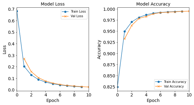
Let’s visualize the model training history by utilizing the toolbox’s
plot_loss, plot_acc, and combine_loss_acc_plots functions.
combine_loss_acc_plots(model_1H_history,
              plot_loss, plot_acc, show=False)
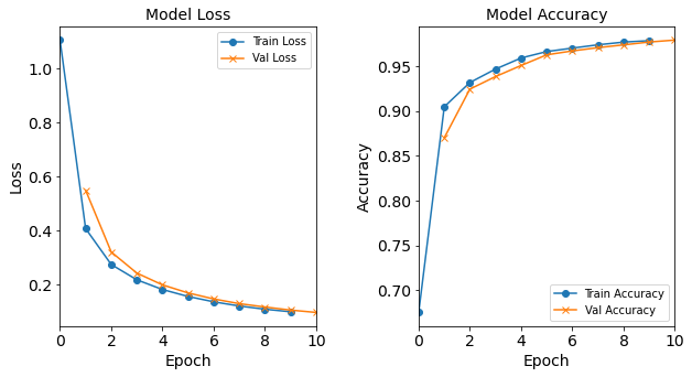
Figure: Loss function and accuracy of the baseline model as a function of epochs (training iterations).
Next, let’s save the model’s outputs using the helper function
saveOutputs_HN.
# Save the outputs
saveOutputs_HN(18, model_1H_history, model_1H)
QUESTION:
What are other adjustable hyperparameters in this model?
Solutions
hidden_neurons(the number of neurons in the hidden layer),epochandbatch_sizeare three important hyperparameters. The activation function can also be considered a hyperparameter that affects the architecture of the model. There are also various other adjustable hyperparameters.
Model Tuning Experiments
Now that we have built and trained the baseline neural network model, we will run a variety of experiments using different combinations of hyperparameters, in order to find the best performing model. Below is a list of hyperparameters that could be interesting to explore; feel free to experiment with your own ideas as well.
We will use the NN_Model_1H with 18 neurons in the hidden layer as a baseline.
Note that the baseline model’s hyperparameter values are listed first
(sequentially) in each category/type of experiment listed below.
Let us:
- Test with different numbers of neurons in the hidden layer: 18, 12, 8, 4, 2, 1
- It is also worthwhile to test a higher number of neurons: 40, 80, or more.
- Test with different learning rates: 0.0003, 0.001, 0.01, 0.1
- Test with different batch sizes: 32, 16, 64, 128, 512, 1024
- Test with different numbers of hidden layers: 1, 2, 3, and so on
NOTE: The easiest way to do this exploration is to simply copy the code cell where we constructed and trained the baseline model and paste it to a new cell below, since most of the parameters (
hidden_neurons,learning_rate,batch_size, etc.) can be changed when calling theNN_Model_1Hfunction or when fitting the model. However, to change the number of hidden layers (which we will do much later), the originalNN_model_1Hfunction must be duplicated and modified.
Model Metadata
While running the experiments on the model, it is imperative that the user collect additional information about each run to assist in the later model tuning phases. This additional data collected is considered metadata. Saving metadata enables the user to quickly recall important information regarding a particular run/experiment. The type of metadata collected depends on what is important for the user to track. For these experiments, we will track how increasing or decreasing one hyperparameter affects the model’s accuracy. For this simplified experiment, we will just track the value of the hyperparameter that is being varied.
This metadata can either be saved during each experiment (this helps ensure that no mistakes are made) or it can be saved after the experiment runs if the user is very careful to remember what to fill in for each run. When creating more experiments, remember to add the appropriate metadata information!
Model Naming Convention
Use systematic names for the model and history variables. The model code used for these experiments follow a naming convention (or short-hand) created as a means of quickly identifying hyperparameter information.
The variable called model_1H12N means “a model with one hidden layer (1H)
that has 12 neurons (12N)”.
The use of systematic names, albeit complicated,
will be very helpful in keeping track of different experiments.
DISCUSSION QUESTIONS: Naming Convention
Why don’t we just name the variables
model1,model2,model3, …? What are the advantages and disadvantages of naming them with this schema?Solution
The disadvantage to using the
model1,model2, etc. naming convention is that the user must keep track (elsewhere) of the metadata information. What if months later you need to investigatemodel1? There would not be a quick way to look up the hyperparameter values. You can gather some of the hyperparameter values from saved information, but using this naming convention will greatly speed up that process.Using a naming convention for the models that include some metadata allows the user to more readily identify the model and identify the hyperparameter values.
We will implement the following naming convention, where the words in all caps
are placeholders for their numerical values (used in that particular model).
Except for the MODEL_NAME which will be replaced with the model code that follows the naming convention.
MODEL_NAME = model_1H + HIDDEN_NEURONS + N_lr + LEARNING_RATE + _bs + BATCH_SIZE + _e + EPOCHS
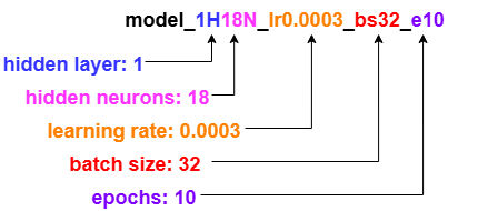
Figure: A visual representation of the naming convention for the baseline model.
Keeping track of experimental results:
At this stage, it may be helpful to keep track of the final training accuracy (the last epoch result)
for each model with a distinct hidden_neurons value.
You can use pen-and-paper, or build a spreadsheet with the following
values:
hidden_neurons |
val_accuracy |
|---|---|
| 1 | …. |
| … | …. |
| 18 | 0.9792 (example) |
| … | …. |
| 80 | …. |
Tuning Experiments, Part 1: Varying Number of Neurons in Hidden Layers
In this round of experiments, we create several variants of NN_Model_1H models
with varying hidden_neurons hyperparameter values,
i.e., the number of neurons in the hidden layer.
Increasing the number of neurons increases the complexity of the model.
Decreasing the number of neurons decreases the complexity of the model.
A more complex model increases the capability of the model
to capture more complex patterns.
The number of neurons can be thought of as the “width” of the hidden layer.
The loss and accuracy of each model will be assessed as a function of hidden_neurons.
All the other hyperparameters (i.e., learning rate, epochs, batch size, number of hidden layers)
will be kept constant; they will be varied later one by one.
Not every number of hidden neurons is tested,
so feel free to create new code cells with a different number of neurons as your curiousity leads you.
Going in FEWER hidden neurons
Model “1H12N”: 12 neurons in the hidden layer
"""Construct & train a NN_Model_1H with 12 neurons in the hidden layer""";

model_1H12N = NN_Model_1H(12,0.0003)
model_1H12N_history = model_1H12N.fit(train_features,
                                      train_L_onehot,
                                      epochs=10, batch_size=32,
                                      validation_data=(test_features, test_L_onehot),
                                      verbose=2)

saveOutputs_HN(12, model_1H12N_history, model_1H12N)
Created model: NN_Model_1H
 - hidden_layers  = 1
 - hidden_neurons = 12
 - optimizer      = Adam
 - learning_rate  = 0.0003

Epoch 1/10
6827/6827 - 7s - loss: 1.1864 - accuracy: 0.6581 - val_loss: 0.6118 - val_accuracy: 0.8622
Epoch 2/10
6827/6827 - 7s - loss: 0.4592 - accuracy: 0.8992 - val_loss: 0.3700 - val_accuracy: 0.9217
Epoch 3/10
6827/6827 - 6s - loss: 0.3286 - accuracy: 0.9277 - val_loss: 0.2997 - val_accuracy: 0.9331
Epoch 4/10
6827/6827 - 6s - loss: 0.2803 - accuracy: 0.9349 - val_loss: 0.2659 - val_accuracy: 0.9381
Epoch 5/10
6827/6827 - 6s - loss: 0.2531 - accuracy: 0.9381 - val_loss: 0.2437 - val_accuracy: 0.9407
Epoch 6/10
6827/6827 - 6s - loss: 0.2328 - accuracy: 0.9413 - val_loss: 0.2253 - val_accuracy: 0.9448
Epoch 7/10
6827/6827 - 6s - loss: 0.2161 - accuracy: 0.9455 - val_loss: 0.2105 - val_accuracy: 0.9507
Epoch 8/10
6827/6827 - 6s - loss: 0.2026 - accuracy: 0.9496 - val_loss: 0.1983 - val_accuracy: 0.9549
Epoch 9/10
6827/6827 - 6s - loss: 0.1908 - accuracy: 0.9540 - val_loss: 0.1871 - val_accuracy: 0.9556
Epoch 10/10
6827/6827 - 6s - loss: 0.1777 - accuracy: 0.9565 - val_loss: 0.1731 - val_accuracy: 0.9593
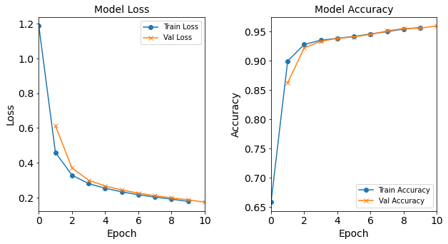
Figure: The model’s loss and accuracy as a function of epochs from the model 1H12N.
Model “1H8N”: 8 neurons in the hidden layer
model_1H8N = NN_Model_1H(8,0.0003)
model_1H8N_history = model_1H8N.fit(train_features,
                                    train_L_onehot,
                                    epochs=10, batch_size=32,
                                    validation_data=(test_features, test_L_onehot),
                                    verbose=2)

saveOutputs_HN(8, model_1H8N_history, model_1H8N)
Created model: NN_Model_1H
 - hidden_layers  = 1
 - hidden_neurons = 8
 - optimizer      = Adam
 - learning_rate  = 0.0003

Epoch 1/10
6827/6827 - 7s - loss: 1.3739 - accuracy: 0.5619 - val_loss: 0.7965 - val_accuracy: 0.7703
Epoch 2/10
6827/6827 - 6s - loss: 0.6197 - accuracy: 0.8551 - val_loss: 0.5010 - val_accuracy: 0.8908
Epoch 3/10
6827/6827 - 6s - loss: 0.4364 - accuracy: 0.9050 - val_loss: 0.3895 - val_accuracy: 0.9152
Epoch 4/10
6827/6827 - 6s - loss: 0.3560 - accuracy: 0.9174 - val_loss: 0.3312 - val_accuracy: 0.9211
Epoch 5/10
6827/6827 - 6s - loss: 0.3123 - accuracy: 0.9234 - val_loss: 0.2988 - val_accuracy: 0.9277
Epoch 6/10
6827/6827 - 6s - loss: 0.2861 - accuracy: 0.9257 - val_loss: 0.2773 - val_accuracy: 0.9229
Epoch 7/10
6827/6827 - 6s - loss: 0.2677 - accuracy: 0.9261 - val_loss: 0.2608 - val_accuracy: 0.9274
Epoch 8/10
6827/6827 - 6s - loss: 0.2529 - accuracy: 0.9296 - val_loss: 0.2470 - val_accuracy: 0.9311
Epoch 9/10
6827/6827 - 6s - loss: 0.2405 - accuracy: 0.9340 - val_loss: 0.2351 - val_accuracy: 0.9328
Epoch 10/10
6827/6827 - 6s - loss: 0.2294 - accuracy: 0.9375 - val_loss: 0.2249 - val_accuracy: 0.9396

Figure: The model’s loss and accuracy as a function of epochs from the model 1H8N.
Exercises
Create additional code cells to run models with 4, 2, 1 neurons in the hidden layer
Model “1H4N”: 4 neurons in the hidden layer
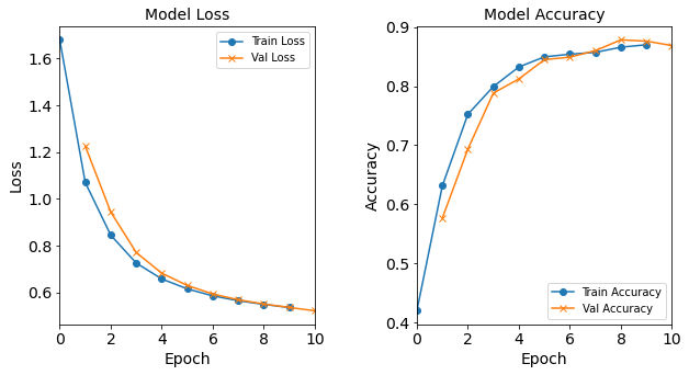
model_1H4N = NN_Model_1H(4,0.0003)
model_1H4N_history = model_1H4N.fit(train_features,
                                    train_L_onehot,
                                    epochs=10, batch_size=32,
                                    validation_data=(test_features, test_L_onehot),
                                    verbose=2)

saveOutputs_HN(4, model_1H4N_history, model_1H4N)
Created model: NN_Model_1H - hidden_layers = 1 - hidden_neurons = 4 - optimizer = Adam - learning_rate = 0.0003 Epoch 1/10 6827/6827 - 8s - loss: 1.6787 - accuracy: 0.4199 - val_loss: 1.2247 - val_accuracy: 0.5768 Epoch 2/10 6827/6827 - 7s - loss: 1.0693 - accuracy: 0.6315 - val_loss: 0.9432 - val_accuracy: 0.6934 Epoch 3/10 6827/6827 - 8s - loss: 0.8440 - accuracy: 0.7524 - val_loss: 0.7699 - val_accuracy: 0.7884 Epoch 4/10 6827/6827 - 8s - loss: 0.7248 - accuracy: 0.7993 - val_loss: 0.6817 - val_accuracy: 0.8122 Epoch 5/10 6827/6827 - 8s - loss: 0.6571 - accuracy: 0.8325 - val_loss: 0.6291 - val_accuracy: 0.8449 Epoch 6/10 6827/6827 - 8s - loss: 0.6146 - accuracy: 0.8495 - val_loss: 0.5927 - val_accuracy: 0.8491 Epoch 7/10 6827/6827 - 8s - loss: 0.5846 - accuracy: 0.8541 - val_loss: 0.5679 - val_accuracy: 0.8601 Epoch 8/10 6827/6827 - 8s - loss: 0.5640 - accuracy: 0.8572 - val_loss: 0.5498 - val_accuracy: 0.8783 Epoch 9/10 6827/6827 - 8s - loss: 0.5483 - accuracy: 0.8659 - val_loss: 0.5352 - val_accuracy: 0.8762 Epoch 10/10 6827/6827 - 8s - loss: 0.5347 - accuracy: 0.8701 - val_loss: 0.5208 - val_accuracy: 0.8687
Figure: The model’s loss and accuracy as a function of epochs from the model 1H4N.
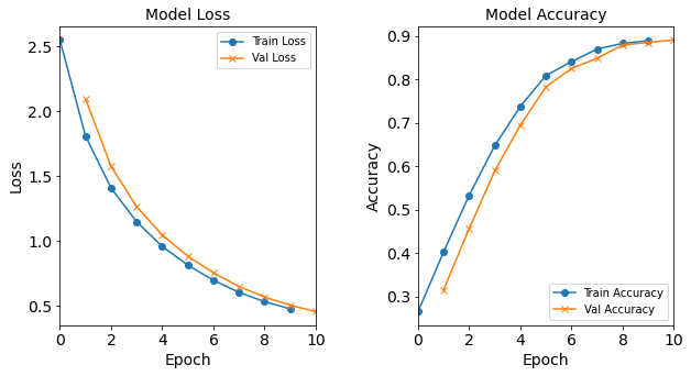
Model “1H2N”: 2 neurons in the hidden layer
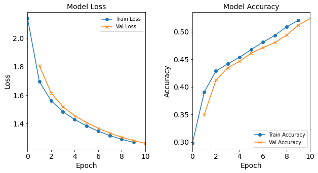
model_1H2N = NN_Model_1H(2,0.0003)
model_1H2N_history = model_1H2N.fit(train_features,
                                    train_L_onehot,
                                    epochs=10, batch_size=32,
                                    validation_data=(test_features, test_L_onehot),
                                    verbose=2)

saveOutputs_HN(2, model_1H2N_history, model_1H2N)
Created model: NN_Model_1H - hidden_layers = 1 - hidden_neurons = 2 - optimizer = Adam - learning_rate = 0.0003 Epoch 1/10 6827/6827 - 9s - loss: 2.1385 - accuracy: 0.2973 - val_loss: 1.8072 - val_accuracy: 0.3491 Epoch 2/10 6827/6827 - 7s - loss: 1.6945 - accuracy: 0.3901 - val_loss: 1.6147 - val_accuracy: 0.4122 Epoch 3/10 6827/6827 - 7s - loss: 1.5603 - accuracy: 0.4286 - val_loss: 1.5186 - val_accuracy: 0.4345 Epoch 4/10 6827/6827 - 7s - loss: 1.4834 - accuracy: 0.4416 - val_loss: 1.4552 - val_accuracy: 0.4462 Epoch 5/10 6827/6827 - 7s - loss: 1.4283 - accuracy: 0.4535 - val_loss: 1.4069 - val_accuracy: 0.4610 Epoch 6/10 6827/6827 - 7s - loss: 1.3843 - accuracy: 0.4677 - val_loss: 1.3668 - val_accuracy: 0.4711 Epoch 7/10 6827/6827 - 7s - loss: 1.3467 - accuracy: 0.4811 - val_loss: 1.3322 - val_accuracy: 0.4803 Epoch 8/10 6827/6827 - 7s - loss: 1.3153 - accuracy: 0.4931 - val_loss: 1.3039 - val_accuracy: 0.4937 Epoch 9/10 6827/6827 - 8s - loss: 1.2892 - accuracy: 0.5089 - val_loss: 1.2802 - val_accuracy: 0.5120 Epoch 10/10 6827/6827 - 7s - loss: 1.2678 - accuracy: 0.5205 - val_loss: 1.2608 - val_accuracy: 0.5241
Figure: The model’s loss and accuracy as a function of epochs from the model 1H2N.
Model “1H1N”: 1 neuron in the hidden layer
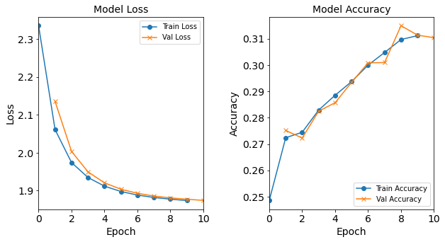
model_1H1N = NN_Model_1H(1,0.0003)
model_1H1N_history = model_1H1N.fit(train_features,
                                    train_L_onehot,
                                    epochs=10, batch_size=32,
                                    validation_data=(test_features, test_L_onehot),
                                    verbose=2)

saveOutputs_HN(1, model_1H1N_history, model_1H1N)
Created model: NN_Model_1H - hidden_layers = 1 - hidden_neurons = 1 - optimizer = Adam - learning_rate = 0.0003 Epoch 1/10 6827/6827 - 8s - loss: 2.3351 - accuracy: 0.2485 - val_loss: 2.1355 - val_accuracy: 0.2752 Epoch 2/10 6827/6827 - 7s - loss: 2.0610 - accuracy: 0.2724 - val_loss: 2.0034 - val_accuracy: 0.2723 Epoch 3/10 6827/6827 - 7s - loss: 1.9741 - accuracy: 0.2745 - val_loss: 1.9494 - val_accuracy: 0.2825 Epoch 4/10 6827/6827 - 7s - loss: 1.9346 - accuracy: 0.2829 - val_loss: 1.9205 - val_accuracy: 0.2857 Epoch 5/10 6827/6827 - 7s - loss: 1.9118 - accuracy: 0.2885 - val_loss: 1.9036 - val_accuracy: 0.2934 Epoch 6/10 6827/6827 - 8s - loss: 1.8976 - accuracy: 0.2937 - val_loss: 1.8930 - val_accuracy: 0.3008 Epoch 7/10 6827/6827 - 7s - loss: 1.8883 - accuracy: 0.3000 - val_loss: 1.8856 - val_accuracy: 0.3009 Epoch 8/10 6827/6827 - 7s - loss: 1.8819 - accuracy: 0.3048 - val_loss: 1.8808 - val_accuracy: 0.3149 Epoch 9/10 6827/6827 - 7s - loss: 1.8774 - accuracy: 0.3097 - val_loss: 1.8772 - val_accuracy: 0.3114 Epoch 10/10 6827/6827 - 8s - loss: 1.8737 - accuracy: 0.3112 - val_loss: 1.8742 - val_accuracy: 0.3104
Figure: The model’s loss and accuracy as a function of epochs from the model 1H1N.
Going in the direction of MORE hidden neurons
Exercises
Create more code cells to run models with 40 and 80 neurons in the hidden layer. You are welcome to explore even higher numbers of hidden neurons. Observe carefully what is happening!
Model “1H4N”: 40 neurons in the hidden layer
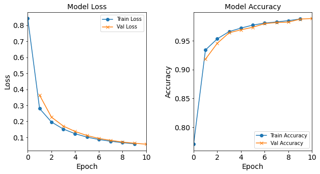
model_1H40N = NN_Model_1H(40,0.0003)
model_1H40N_history = model_1H40N.fit(train_features,
                                      train_L_onehot,
                                      epochs=10, batch_size=32,
                                      validation_data=(test_features, test_L_onehot),
                                      verbose=2)

saveOutputs_HN(40, model_1H40N_history, model_1H40N)
Created model: NN_Model_1H - hidden_layers = 1 - hidden_neurons = 40 - optimizer = Adam - learning_rate = 0.0003 Epoch 1/10 6827/6827 - 9s - loss: 0.8427 - accuracy: 0.7706 - val_loss: 0.3632 - val_accuracy: 0.9180 Epoch 2/10 6827/6827 - 9s - loss: 0.2798 - accuracy: 0.9339 - val_loss: 0.2265 - val_accuracy: 0.9456 Epoch 3/10 6827/6827 - 9s - loss: 0.1958 - accuracy: 0.9533 - val_loss: 0.1706 - val_accuracy: 0.9637 Epoch 4/10 6827/6827 - 9s - loss: 0.1519 - accuracy: 0.9658 - val_loss: 0.1364 - val_accuracy: 0.9689 Epoch 5/10 6827/6827 - 9s - loss: 0.1226 - accuracy: 0.9718 - val_loss: 0.1113 - val_accuracy: 0.9733 Epoch 6/10 6827/6827 - 9s - loss: 0.1014 - accuracy: 0.9770 - val_loss: 0.0931 - val_accuracy: 0.9796 Epoch 7/10 6827/6827 - 9s - loss: 0.0864 - accuracy: 0.9805 - val_loss: 0.0810 - val_accuracy: 0.9815 Epoch 8/10 6827/6827 - 9s - loss: 0.0755 - accuracy: 0.9825 - val_loss: 0.0704 - val_accuracy: 0.9822 Epoch 9/10 6827/6827 - 9s - loss: 0.0667 - accuracy: 0.9848 - val_loss: 0.0632 - val_accuracy: 0.9874 Epoch 10/10 6827/6827 - 9s - loss: 0.0596 - accuracy: 0.9875 - val_loss: 0.0570 - val_accuracy: 0.9884
Figure: The model’s loss and accuracy as a function of epochs from the model 1H40N.
Model “1H80N”: 80 neurons in the hidden layer
model_1H80N = NN_Model_1H(80,0.0003)
model_1H80N_history = model_1H80N.fit(train_features,
                                      train_L_onehot,
                                      epochs=10, batch_size=32,
                                      validation_data=(test_features, test_L_onehot),
                                      verbose=2)

saveOutputs_HN(80, model_1H80N_history, model_1H80N)
Created model: NN_Model_1H - hidden_layers = 1 - hidden_neurons = 80 - optimizer = Adam - learning_rate = 0.0003 Epoch 1/10 6827/6827 - 9s - loss: 0.6815 - accuracy: 0.8244 - val_loss: 0.2710 - val_accuracy: 0.9327 Epoch 2/10 6827/6827 - 9s - loss: 0.2048 - accuracy: 0.9492 - val_loss: 0.1580 - val_accuracy: 0.9629 Epoch 3/10 >> 6827/6827 - 9s - loss: 0.1291 - accuracy: 0.9708 - val_loss: 0.1058 - val_accuracy: 0.9786 Epoch 4/10 6827/6827 - 9s - loss: 0.0900 - accuracy: 0.9808 - val_loss: 0.0764 - val_accuracy: 0.9829 Epoch 5/10 6827/6827 - 9s - loss: 0.0669 - accuracy: 0.9865 - val_loss: 0.0587 - val_accuracy: 0.9888 Epoch 6/10 6827/6827 - 9s - loss: 0.0525 - accuracy: 0.9902 - val_loss: 0.0463 - val_accuracy: 0.9915 Epoch 7/10 6827/6827 - 9s - loss: 0.0424 - accuracy: 0.9919 - val_loss: 0.0377 - val_accuracy: 0.9925 Epoch 8/10 6827/6827 - 9s - loss: 0.0351 - accuracy: 0.9931 - val_loss: 0.0326 - val_accuracy: 0.9933 Epoch 9/10 6827/6827 - 9s - loss: 0.0299 - accuracy: 0.9939 - val_loss: 0.0282 - val_accuracy: 0.9943 Epoch 10/10 6827/6827 - 9s - loss: 0.0258 - accuracy: 0.9945 - val_loss: 0.0244 - val_accuracy: 0.9948
Figure: The model’s loss and accuracy as a function of epochs from the model 1H80N.
Post-Processing from Tuning Experiments Part 1: Hidden Neurons
In the first experiment above, we tuned the NN_Model_1H model
by varying only the hidden_neurons hyperparameter.
Post-processing consists of the following steps.
Step 1: Discovering the results. This step consists of running the models and saving the outputs as variables.
Step 2: Validating the data. This step is completed by using the visualizations of the model training history. To take advantage of Jupyter Notebook’s ability to immediately inspect graphical elements, this step should be done after each model run.
-
Visually inspect for any anomalies. Do any of the graphs exhibit different behavior than what is shown in the baseline model graphs?
-
Visually or numerically check for convergence (e.g., check the last 4-5 epochs, what the slope is like; any fluctuations?).
-
Observe the differences in the final accuracies as a result of varying the hyperparameter values.
Step 3: Saving the results. This step consists of collecting the output variables, creating a DataFrame to hold all the metadata and output information (i.e., last epoch metrics, such as accuracy), and saving this DataFrame to a CSV file (a comma-separated values text file format used to store tabular data). A DataFrame is a Pandas data structure similar to a table with rows and columns.
Though there are multiple ways of conducting step 3, we will construct and fill a temporary data structure dynamically before formatting the dataframe. This approach is useful when the size of the data (i.e., total number of rows) is not known a priori.
Post-Processing Results for the Hidden Neurons Experiment
The resulting accuracy graph for the model with 1 hidden neuron does not appear to converge (and does not follow the typical trend). The resulting accuracy graph for the model with 2 hidden neurons does not appear to follow the typical trend, though it does appear to start to converge.
# outer directory
dirPathHN = dir0_HN

# The number of neurons for each experiment/model
listHN = [1, 2, 4, 8, 12, 18, 40, 80] # change this line to reflect the experiments you did run!

# Number of epochs - 1
lastEpochNum = 9

# Initalize. This will hold the list of dictionaries of last epoch metrics
# (loss, val_loss, accuracy, val_accuracy)
all_lastEpochMetrics = []

# Fill in the rows for the DataFrame
for HN in listHN:
    # Read the history CSV file and get the last row's data, which corresponds to the last epoch data.
    result_csv = fn_out_history_1H(dirPathHN, HN, 0.0003, 32, 10)
    print("Reading:", result_csv)
    epochMetrics = pd.read_csv(result_csv)
    # Fetch the loss, accuracy, val_loss, and val_accuracy from the last epoch
    # (should be the last row in the CSV file unless there's something wrong
    # during the traning)
    lastEpochMetrics = epochMetrics.iloc[lastEpochNum, :].to_dict()
    # Attach the "neurons" value
    lastEpochMetrics["hidden_neurons"] = HN
    all_lastEpochMetrics.append(lastEpochMetrics)
   hidden_neurons      loss  accuracy  val_loss  val_accuracy
0               1  1.873713  0.311159  1.874192      0.310367
1               2  1.267804  0.520468  1.260848      0.524095
2               4  0.534735  0.870068  0.520849      0.868701
3               8  0.274668  0.934126  0.273426      0.936154
4              12  0.177680  0.956532  0.173094      0.959279
5              18  0.099545  0.978559  0.097021      0.979219
6              40  0.059567  0.987522  0.057018      0.988447
7              80  0.025805  0.994502  0.024440      0.994800
Save the post-processing results for the hidden neurons experiment.
df_HN.to_csv("post_processing_neurons.csv", index=False)
A later episode discusses the post-analysis from this and subsequent experiments in this episode. Post-analysis begins with loading in the CSV file that contains the DataFrame of the model metadata and model outputs. Then, by creating a plot showing how the model’s accuracy is affected by one hyperparameter. This visualization is then used to draw conclusions and hypotheses that can be used to find a more ideal value for the hyperparameter.
Tuning Experiments, Part 2: Varying Learning Rate
In this batch of experiments, we will observe how increasing or decreasing just the learning rate hyperparameter affects the model’s accuracy. For simplicity, all the other parameters (i.e., the number of neurons, epochs, batch size, and hidden layers) will be kept constant. The initial Baseline model will also be included. Not every learning rate is tested, so feel free to create new code cells with a different learning rate. Recall that learning rate determines the “step size” or amount that the model is able to change after each iteration.
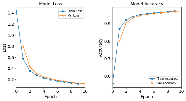
Model “1H18N” With Learning Rate 0.0003
model_1H18N_LR0_0003 = NN_Model_1H(18,0.0003)
model_1H18N_LR0_0003_history = model_1H18N_LR0_0003.fit(train_features,
                                                        train_L_onehot,
                                                        epochs=10, batch_size=32,
                                                        validation_data=(test_features, test_L_onehot),
                                                        verbose=2)

saveOutputs_LR(0.0003, model_1H18N_LR0_0003_history, model_1H18N_LR0_0003)
Created model: NN_Model_1H
 - hidden_layers  = 1
 - hidden_neurons = 18
 - optimizer      = Adam
 - learning_rate  = 0.0003
Epoch 1/10
6827/6827 - 11s - loss: 1.1029 - accuracy: 0.6803 - val_loss: 0.5063 - val_accuracy: 0.8949
Epoch 2/10
6827/6827 - 10s - loss: 0.3616 - accuracy: 0.9233 - val_loss: 0.2791 - val_accuracy: 0.9413
Epoch 3/10
6827/6827 - 10s - loss: 0.2377 - accuracy: 0.9498 - val_loss: 0.2081 - val_accuracy: 0.9534
Epoch 4/10
6827/6827 - 10s - loss: 0.1850 - accuracy: 0.9585 - val_loss: 0.1678 - val_accuracy: 0.9620
Epoch 5/10
6827/6827 - 10s - loss: 0.1517 - accuracy: 0.9653 - val_loss: 0.1397 - val_accuracy: 0.9675
Epoch 6/10
6827/6827 - 10s - loss: 0.1287 - accuracy: 0.9705 - val_loss: 0.1209 - val_accuracy: 0.9725
Epoch 7/10
6827/6827 - 10s - loss: 0.1129 - accuracy: 0.9741 - val_loss: 0.1079 - val_accuracy: 0.9737
Epoch 8/10
6827/6827 - 10s - loss: 0.1016 - accuracy: 0.9758 - val_loss: 0.0982 - val_accuracy: 0.9770
Epoch 9/10
6827/6827 - 9s - loss: 0.0929 - accuracy: 0.9772 - val_loss: 0.0905 - val_accuracy: 0.9770
Epoch 10/10
6827/6827 - 10s - loss: 0.0859 - accuracy: 0.9787 - val_loss: 0.0847 - val_accuracy: 0.9788
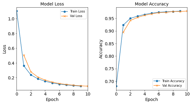
Figure: The model’s loss and accuracy as a function of epochs from the model 1H18N_lr0.0003.
Exercises
Create additional code cells to run models (
1H18N) with larger learning rates: 0.001, 0.01,0.1Model “1H18N” with Learning Rate 0.001
model_1H18N_LR0_001 = NN_Model_1H(18,0.001)
model_1H18N_LR0_001_history = model_1H18N_LR0_001.fit(train_features,
                                      train_L_onehot,
                                      epochs=10, batch_size=32,
                                      validation_data=(test_features, test_L_onehot),
                                      verbose=2)

saveOutputs_LR(0.001, model_1H18N_LR0_001_history, model_1H18N_LR0_001)
Created model: NN_Model_1H - hidden_layers = 1 - hidden_neurons = 18 - optimizer = Adam - learning_rate = 0.001 Epoch 1/10 6827/6827 - 6s - loss: 0.5687 - accuracy: 0.8485 - val_loss: 0.2241 - val_accuracy: 0.9488 Epoch 2/10 6827/6827 - 6s - loss: 0.1676 - accuracy: 0.9621 - val_loss: 0.1305 - val_accuracy: 0.9677 Epoch 3/10 6827/6827 - 6s - loss: 0.1106 - accuracy: 0.9740 - val_loss: 0.0954 - val_accuracy: 0.9750 Epoch 4/10 6827/6827 - 6s - loss: 0.0856 - accuracy: 0.9785 - val_loss: 0.0769 - val_accuracy: 0.9804 Epoch 5/10 6827/6827 - 6s - loss: 0.0712 - accuracy: 0.9827 - val_loss: 0.0656 - val_accuracy: 0.9829 Epoch 6/10 6827/6827 - 6s - loss: 0.0607 - accuracy: 0.9860 - val_loss: 0.0548 - val_accuracy: 0.9886 Epoch 7/10 6827/6827 - 6s - loss: 0.0523 - accuracy: 0.9884 - val_loss: 0.0507 - val_accuracy: 0.9893 Epoch 8/10 6827/6827 - 6s - loss: 0.0467 - accuracy: 0.9896 - val_loss: 0.0450 - val_accuracy: 0.9891 Epoch 9/10 6827/6827 - 7s - loss: 0.0418 - accuracy: 0.9903 - val_loss: 0.0402 - val_accuracy: 0.9902 Epoch 10/10 6827/6827 - 6s - loss: 0.0381 - accuracy: 0.9912 - val_loss: 0.0364 - val_accuracy: 0.9921
Figure: The model’s loss and accuracy as a function of epochs from the model 1H18N_lr0.001.
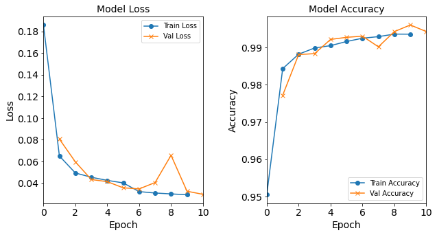
Model “1H18N” with Learning Rate 0.01
model_1H18N_LR0_01 = NN_Model_1H(18,0.01)
model_1H18N_LR0_01_history = model_1H18N_LR0_01.fit(train_features,
                                      train_L_onehot,
                                      epochs=10, batch_size=32,
                                      validation_data=(test_features, test_L_onehot),
                                      verbose=2)

saveOutputs_LR(0.01, model_1H18N_LR0_01_history, model_1H18N_LR0_01)
Created model: NN_Model_1H - hidden_layers = 1 - hidden_neurons = 18 - optimizer = Adam - learning_rate = 0.01 Epoch 1/10 6827/6827 - 6s - loss: 0.1862 - accuracy: 0.9504 - val_loss: 0.0835 - val_accuracy: 0.9769 Epoch 2/10 6827/6827 - 6s - loss: 0.0659 - accuracy: 0.9841 - val_loss: 0.0459 - val_accuracy: 0.9903 Epoch 3/10 6827/6827 - 6s - loss: 0.0500 - accuracy: 0.9884 - val_loss: 0.0506 - val_accuracy: 0.9860 Epoch 4/10 6827/6827 - 6s - loss: 0.0428 - accuracy: 0.9899 - val_loss: 0.0575 - val_accuracy: 0.9907 Epoch 5/10 6827/6827 - 6s - loss: 0.0395 - accuracy: 0.9904 - val_loss: 0.0441 - val_accuracy: 0.9919 Epoch 6/10 6827/6827 - 6s - loss: 0.0381 - accuracy: 0.9918 - val_loss: 0.0311 - val_accuracy: 0.9936 Epoch 7/10 6827/6827 - 6s - loss: 0.0354 - accuracy: 0.9919 - val_loss: 0.0367 - val_accuracy: 0.9894 Epoch 8/10 6827/6827 - 6s - loss: 0.0333 - accuracy: 0.9924 - val_loss: 0.0276 - val_accuracy: 0.9931 Epoch 9/10 6827/6827 - 6s - loss: 0.0312 - accuracy: 0.9927 - val_loss: 0.0227 - val_accuracy: 0.9954 Epoch 10/10 6827/6827 - 6s - loss: 0.0334 - accuracy: 0.9932 - val_loss: 0.0349 - val_accuracy: 0.9915
Figure: The model’s loss and accuracy as a function of epochs from the model 1H18N_lr0.01.
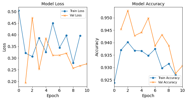
Model “1H18N” with Learning Rate 0.1
model_1H18N_LR0_1 = NN_Model_1H(18,0.1)
model_1H18N_LR0_1_history = model_1H18N_LR0_1.fit(train_features,
                                      train_L_onehot,
                                      epochs=10, batch_size=32,
                                      validation_data=(test_features, test_L_onehot),
                                      verbose=2)

saveOutputs_LR(0.1, model_1H18N_LR0_1_history, model_1H18N_LR0_1)
Created model: NN_Model_1H - hidden_layers = 1 - hidden_neurons = 18 - optimizer = Adam - learning_rate = 0.1 Epoch 1/10 6827/6827 - 6s - loss: 0.4806 - accuracy: 0.9238 - val_loss: 0.2683 - val_accuracy: 0.9397 Epoch 2/10 6827/6827 - 6s - loss: 0.2867 - accuracy: 0.9343 - val_loss: 0.2972 - val_accuracy: 0.9402 Epoch 3/10 6827/6827 - 6s - loss: 0.4591 - accuracy: 0.9364 - val_loss: 0.2503 - val_accuracy: 0.9670 Epoch 4/10 6827/6827 - 6s - loss: 0.5727 - accuracy: 0.9405 - val_loss: 0.9521 - val_accuracy: 0.9330 Epoch 5/10 6827/6827 - 6s - loss: 0.3540 - accuracy: 0.9367 - val_loss: 0.2588 - val_accuracy: 0.9394 Epoch 6/10 6827/6827 - 6s - loss: 0.3486 - accuracy: 0.9334 - val_loss: 0.4348 - val_accuracy: 0.9317 Epoch 7/10 6827/6827 - 6s - loss: 0.4706 - accuracy: 0.9351 - val_loss: 0.3515 - val_accuracy: 0.9147 Epoch 8/10 6827/6827 - 6s - loss: 0.3282 - accuracy: 0.9322 - val_loss: 0.2421 - val_accuracy: 0.9375 Epoch 9/10 6827/6827 - 6s - loss: 0.3283 - accuracy: 0.9327 - val_loss: 0.3710 - val_accuracy: 0.9440 Epoch 10/10 6827/6827 - 6s - loss: 0.3883 - accuracy: 0.9245 - val_loss: 0.2722 - val_accuracy: 0.9346
Figure: The model’s loss and accuracy as a function of epochs from the model 1H18N_lr0.1.
Post-Processing: Varying Learning Rate
This is implemented in the same manner as earlier.
Both resulting graphs from the models with 0.01 and 0.1 learning rates do not follow the typical trends. The 0.1 learning rate model deviates a lot from the typical loss and accuracy plot trends!
# outer directory
dirPathLR = dir0_LR

# The learning rates for each experiment/model
listLR = [.0003, 0.001, 0.01, 0.1] # change this line to reflect the experiments you did run!

# Number of epochs - 1
lastEpochNum = 9

# Initalize. This will hold the list of dictionaries of last epoch metrics
# (loss, val_loss, accuracy, val_accuracy)
all_lastEpochMetrics_LR = []

# Fill in the rows for the DataFrame
for LR in listLR:
    # Read the history CSV file and get the last row's data, which corresponds to the last epoch data.
    result_csv = fn_out_history_1H(dirPathLR, 18, LR, 32, lastEpochNum+1)
    print("Reading:", result_csv)
    epochMetrics = pd.read_csv(result_csv)
    # Fetch the loss, accuracy, val_loss, and val_accuracy from the last epoch
    # (should be the last row in the CSV file unless there's something wrong
    # during the traning)
    lastEpochMetrics = epochMetrics.iloc[lastEpochNum, :].to_dict()
    # Attach the "learning rate" value
    lastEpochMetrics["learning_rate"] = LR
    all_lastEpochMetrics_LR.append(lastEpochMetrics)

df_LR = pd.DataFrame(all_lastEpochMetrics_LR,
                     columns=["learning_rate", "loss", "accuracy", "val_loss", "val_accuracy"])
print(df_LR)

df_LR.to_csv("post_processing_lr.csv", index=False)
   learning_rate      loss  accuracy  val_loss  val_accuracy
0         0.0003  0.085931  0.978687  0.084746      0.978816
1         0.0010  0.038100  0.991234  0.036374      0.992090
2         0.0100  0.023799  0.994466  0.020586      0.995001
3         0.1000  0.388289  0.924485  0.272247      0.934598
Tuning Experiments, Part 3: Varying Batch Size
In these experiments, the hyperparameter changing is the batch size. For simplicity, all other parameters (i.e., learning rate, epochs, number of neurons, number of hidden layers) will be kept constant. The Baseline model will be included. Not every batch size is tested, so feel free to create new code cells with different batch sizes. Recall that batch size is a hyperparameter that sets the number of samples used before updating the model.
model_1H18N_BS16 = NN_Model_1H(18,0.0003)
model_1H18N_BS16_history = model_1H18N_BS16.fit(train_features,
                                      train_L_onehot,
                                      epochs=10, batch_size=16,
                                      validation_data=(test_features, test_L_onehot),
                                      verbose=2)

saveOutputs_BS(16, model_1H18N_BS16_history, model_1H18N_BS16)
Created model: NN_Model_1H
 - hidden_layers  = 1
 - hidden_neurons = 18
 - optimizer      = Adam
 - learning_rate  = 0.0003
Epoch 1/10
13654/13654 - 12s - loss: 0.8238 - accuracy: 0.7727 - val_loss: 0.3321 - val_accuracy: 0.9270
Epoch 2/10
13654/13654 - 12s - loss: 0.2556 - accuracy: 0.9389 - val_loss: 0.2078 - val_accuracy: 0.9495
Epoch 3/10
13654/13654 - 12s - loss: 0.1765 - accuracy: 0.9567 - val_loss: 0.1512 - val_accuracy: 0.9634
Epoch 4/10
13654/13654 - 12s - loss: 0.1350 - accuracy: 0.9688 - val_loss: 0.1211 - val_accuracy: 0.9720
Epoch 5/10
13654/13654 - 12s - loss: 0.1113 - accuracy: 0.9748 - val_loss: 0.1021 - val_accuracy: 0.9773
Epoch 6/10
13654/13654 - 12s - loss: 0.0962 - accuracy: 0.9792 - val_loss: 0.0899 - val_accuracy: 0.9811
Epoch 7/10
13654/13654 - 12s - loss: 0.0850 - accuracy: 0.9815 - val_loss: 0.0809 - val_accuracy: 0.9824
Epoch 8/10
13654/13654 - 12s - loss: 0.0767 - accuracy: 0.9829 - val_loss: 0.0734 - val_accuracy: 0.9826
Epoch 9/10
13654/13654 - 12s - loss: 0.0700 - accuracy: 0.9846 - val_loss: 0.0679 - val_accuracy: 0.9862
Epoch 10/10
13654/13654 - 12s - loss: 0.0647 - accuracy: 0.9862 - val_loss: 0.0639 - val_accuracy: 0.9836
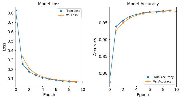
Figure: The model’s loss and accuracy as a function of epochs from the model 1H18N_bs16.
Exercises
Create additional code cells to run models (
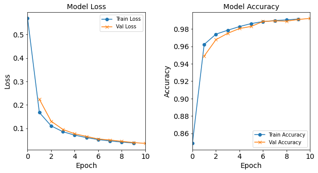
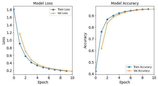
1H18N) with larger batch sizes, (e.g. 16, 32, 64, 128, 512, 1024, …). Remember that we just did an experiment with a batch size = 16.Model “1H18N” With Batch Size 32
model_1H18N_BS32 = NN_Model_1H(18,0.0003)
model_1H18N_BS32_history = model_1H18N_BS32.fit(train_features,
                                      train_L_onehot,
                                      epochs=10, batch_size=32,
                                      validation_data=(test_features, test_L_onehot),
                                      verbose=2)

saveOutputs_BS(32, model_1H18N_BS32_history, model_1H18N_BS32)
Created model: NN_Model_1H - hidden_layers = 1 - hidden_neurons = 18 - optimizer = Adam - learning_rate = 0.0003 Epoch 1/10 6827/6827 - 7s - loss: 1.1029 - accuracy: 0.6803 - val_loss: 0.5063 - val_accuracy: 0.8949 Epoch 2/10 6827/6827 - 6s - loss: 0.3616 - accuracy: 0.9233 - val_loss: 0.2791 - val_accuracy: 0.9413 Epoch 3/10 6827/6827 - 6s - loss: 0.2377 - accuracy: 0.9498 - val_loss: 0.2081 - val_accuracy: 0.9534 Epoch 4/10 6827/6827 - 6s - loss: 0.1850 - accuracy: 0.9585 - val_loss: 0.1679 - val_accuracy: 0.9620 Epoch 5/10 6827/6827 - 6s - loss: 0.1517 - accuracy: 0.9653 - val_loss: 0.1397 - val_accuracy: 0.9676 Epoch 6/10 6827/6827 - 6s - loss: 0.1287 - accuracy: 0.9705 - val_loss: 0.1209 - val_accuracy: 0.9725 Epoch 7/10 6827/6827 - 6s - loss: 0.1129 - accuracy: 0.9741 - val_loss: 0.1079 - val_accuracy: 0.9736 Epoch 8/10 6827/6827 - 6s - loss: 0.1016 - accuracy: 0.9757 - val_loss: 0.0982 - val_accuracy: 0.9770 Epoch 9/10 6827/6827 - 6s - loss: 0.0929 - accuracy: 0.9772 - val_loss: 0.0905 - val_accuracy: 0.9770 Epoch 10/10 6827/6827 - 6s - loss: 0.0859 - accuracy: 0.9787 - val_loss: 0.0847 - val_accuracy: 0.9788
Figure: The model’s loss and accuracy as a function of epochs from the model 1H18N_bs32.
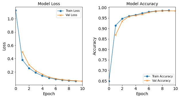
Model “1H18N” With Batch Size 64
model_1H18N_BS64 = NN_Model_1H(18,0.0003)
model_1H18N_BS64_history = model_1H18N_BS64.fit(train_features,
                                      train_L_onehot,
                                      epochs=10, batch_size=64,
                                      validation_data=(test_features, test_L_onehot),
                                      verbose=2)

saveOutputs_BS(64, model_1H18N_BS64_history, model_1H18N_BS64)
Created model: NN_Model_1H - hidden_layers = 1 - hidden_neurons = 18 - optimizer = Adam - learning_rate = 0.0003 Epoch 1/10 3414/3414 - 4s - loss: 1.4388 - accuracy: 0.5565 - val_loss: 0.8041 - val_accuracy: 0.7991 Epoch 2/10 3414/3414 - 3s - loss: 0.5776 - accuracy: 0.8707 - val_loss: 0.4256 - val_accuracy: 0.9052 Epoch 3/10 3414/3414 - 3s - loss: 0.3546 - accuracy: 0.9216 - val_loss: 0.3060 - val_accuracy: 0.9325 Epoch 4/10 3414/3414 - 4s - loss: 0.2738 - accuracy: 0.9401 - val_loss: 0.2500 - val_accuracy: 0.9453 Epoch 5/10 3414/3414 - 3s - loss: 0.2294 - accuracy: 0.9504 - val_loss: 0.2141 - val_accuracy: 0.9519 Epoch 6/10 3414/3414 - 3s - loss: 0.1987 - accuracy: 0.9556 - val_loss: 0.1875 - val_accuracy: 0.9568 Epoch 7/10 3414/3414 - 3s - loss: 0.1750 - accuracy: 0.9597 - val_loss: 0.1665 - val_accuracy: 0.9612 Epoch 8/10 3414/3414 - 3s - loss: 0.1554 - accuracy: 0.9637 - val_loss: 0.1490 - val_accuracy: 0.9654 Epoch 9/10 3414/3414 - 3s - loss: 0.1397 - accuracy: 0.9671 - val_loss: 0.1349 - val_accuracy: 0.9674 Epoch 10/10 3414/3414 - 3s - loss: 0.1271 - accuracy: 0.9715 - val_loss: 0.1236 - val_accuracy: 0.9723
Figure: The model’s loss and accuracy as a function of epochs from the model 1H18N_bs64.
Model “1H18N” With Batch Size 128
model_1H18N_BS128 = NN_Model_1H(18,0.0003)
model_1H18N_BS128_history = model_1H18N_BS128.fit(train_features,
                                      train_L_onehot,
                                      epochs=10, batch_size=128,
                                      validation_data=(test_features, test_L_onehot),
                                      verbose=2)

saveOutputs_BS(128, model_1H18N_BS128_history, model_1H18N_BS128)
Created model: NN_Model_1H - hidden_layers = 1 - hidden_neurons = 18 - optimizer = Adam - learning_rate = 0.0003 Epoch 1/10 1707/1707 - 2s - loss: 1.8142 - accuracy: 0.4222 - val_loss: 1.1781 - val_accuracy: 0.6166 Epoch 2/10 1707/1707 - 2s - loss: 0.9118 - accuracy: 0.7627 - val_loss: 0.7089 - val_accuracy: 0.8346 Epoch 3/10 1707/1707 - 2s - loss: 0.5814 - accuracy: 0.8680 - val_loss: 0.4835 - val_accuracy: 0.8870 Epoch 4/10 1707/1707 - 2s - loss: 0.4178 - accuracy: 0.8995 - val_loss: 0.3700 - val_accuracy: 0.9097 Epoch 5/10 1707/1707 - 2s - loss: 0.3344 - accuracy: 0.9209 - val_loss: 0.3081 - val_accuracy: 0.9280 Epoch 6/10 1707/1707 - 2s - loss: 0.2854 - accuracy: 0.9337 - val_loss: 0.2688 - val_accuracy: 0.9384 Epoch 7/10 1707/1707 - 2s - loss: 0.2521 - accuracy: 0.9426 - val_loss: 0.2398 - val_accuracy: 0.9471 Epoch 8/10 1707/1707 - 2s - loss: 0.2262 - accuracy: 0.9491 - val_loss: 0.2164 - val_accuracy: 0.9505 Epoch 9/10 1707/1707 - 2s - loss: 0.2052 - accuracy: 0.9528 - val_loss: 0.1972 - val_accuracy: 0.9536 Epoch 10/10 1707/1707 - 2s - loss: 0.1879 - accuracy: 0.9550 - val_loss: 0.1814 - val_accuracy: 0.9551
Figure: The model’s loss and accuracy as a function of epochs from the model 1H18N_bs128.
Model “1H18N” With Batch Size 512
model_1H18N_BS512 = NN_Model_1H(18,0.0003)
model_1H18N_BS512_history = model_1H18N_BS512.fit(train_features,
                                      train_L_onehot,
                                      epochs=10, batch_size=512,
                                      validation_data=(test_features, test_L_onehot),
                                      verbose=2)

saveOutputs_BS(512, model_1H18N_BS512_history, model_1H18N_BS512)
Created model: NN_Model_1H - hidden_layers = 1 - hidden_neurons = 18 - optimizer = Adam - learning_rate = 0.0003 Epoch 1/10 427/427 - 1s - loss: 2.5478 - accuracy: 0.2648 - val_loss: 2.0955 - val_accuracy: 0.3152 Epoch 2/10 427/427 - 1s - loss: 1.8088 - accuracy: 0.4025 - val_loss: 1.5753 - val_accuracy: 0.4566 Epoch 3/10 427/427 - 1s - loss: 1.4084 - accuracy: 0.5331 - val_loss: 1.2653 - val_accuracy: 0.5890 Epoch 4/10 427/427 - 1s - loss: 1.1491 - accuracy: 0.6474 - val_loss: 1.0477 - val_accuracy: 0.6946 Epoch 5/10 427/427 - 1s - loss: 0.9598 - accuracy: 0.7376 - val_loss: 0.8844 - val_accuracy: 0.7828 Epoch 6/10 427/427 - 1s - loss: 0.8154 - accuracy: 0.8087 - val_loss: 0.7568 - val_accuracy: 0.8250 Epoch 7/10 427/427 - 1s - loss: 0.6995 - accuracy: 0.8407 - val_loss: 0.6515 - val_accuracy: 0.8484 Epoch 8/10 427/427 - 1s - loss: 0.6063 - accuracy: 0.8697 - val_loss: 0.5704 - val_accuracy: 0.8790 Epoch 9/10 427/427 - 1s - loss: 0.5349 - accuracy: 0.8828 - val_loss: 0.5077 - val_accuracy: 0.8848 Epoch 10/10 427/427 - 1s - loss: 0.4792 - accuracy: 0.8887 - val_loss: 0.4581 - val_accuracy: 0.8906
Figure: The model’s loss and accuracy as a function of epochs from the model 1H18N_bs512.
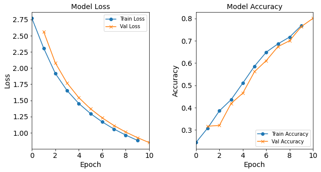
Model “1H18N” With Batch Size 1024
model_1H18N_BS1024 = NN_Model_1H(18,0.0003)
model_1H18N_BS1024_history = model_1H18N_BS1024.fit(train_features,
                                      train_L_onehot,
                                      epochs=10, batch_size=1024,
                                      validation_data=(test_features, test_L_onehot),
                                      verbose=2)

saveOutputs_BS(1024, model_1H18N_BS1024_history, model_1H18N_BS1024)
Created model: NN_Model_1H - hidden_layers = 1 - hidden_neurons = 18 - optimizer = Adam - learning_rate = 0.0003 Epoch 1/10 214/214 - 1s - loss: 2.7688 - accuracy: 0.2434 - val_loss: 2.5636 - val_accuracy: 0.3167 Epoch 2/10 214/214 - 0s - loss: 2.3085 - accuracy: 0.3085 - val_loss: 2.0787 - val_accuracy: 0.3201 Epoch 3/10 214/214 - 0s - loss: 1.9158 - accuracy: 0.3856 - val_loss: 1.7679 - val_accuracy: 0.4188 Epoch 4/10 214/214 - 1s - loss: 1.6514 - accuracy: 0.4357 - val_loss: 1.5421 - val_accuracy: 0.4649 Epoch 5/10 214/214 - 0s - loss: 1.4515 - accuracy: 0.5100 - val_loss: 1.3691 - val_accuracy: 0.5613 Epoch 6/10 214/214 - 0s - loss: 1.2958 - accuracy: 0.5860 - val_loss: 1.2295 - val_accuracy: 0.6109 Epoch 7/10 214/214 - 1s - loss: 1.1667 - accuracy: 0.6487 - val_loss: 1.1110 - val_accuracy: 0.6735 Epoch 8/10 214/214 - 0s - loss: 1.0568 - accuracy: 0.6860 - val_loss: 1.0103 - val_accuracy: 0.7002 Epoch 9/10 214/214 - 0s - loss: 0.9632 - accuracy: 0.7167 - val_loss: 0.9237 - val_accuracy: 0.7638 Epoch 10/10 214/214 - 0s - loss: 0.8815 - accuracy: 0.7684 - val_loss: 0.8473 - val_accuracy: 0.8006
Figure: The model’s loss and accuracy as a function of epochs from the model 1H18N_bs1024.

Post-Processing: Varying Batch Size
Run post-processing for the batch size experiments, similar to prior post-processing.
The resulting loss and acccuracy graphs for the model with a batch size of 512 starts to deviate from the typical trends. The resulting accuracy (and loss) graphs for the model with a batch size of 1024 starts to really diviate from the typical trends.
# outer directory
dirPathLR = dir0_BS

# The batch sizes for each experiment/model
listBS = [16, 32, 64, 128, 512, 1024] # change this line to reflect the experiments you did run!

# Number of epochs - 1
lastEpochNum = 9

# Initalize. This will hold the list of dictionaries of last epoch metrics
# (loss, val_loss, accuracy, val_accuracy)
all_lastEpochMetrics_BS = []

# Fill in the rows for the DataFrame
for BS in listBS:
    # Read the history CSV file and get the last row's data, which corresponds to the last epoch data.
    result_csv = fn_out_history_1H(dirPathLR, 18, 0.0003, BS, lastEpochNum+1)
    print("Reading:", result_csv)
    epochMetrics = pd.read_csv(result_csv)
    # Fetch the loss, accuracy, val_loss, and val_accuracy from the last epoch
    # (should be the last row in the CSV file unless there's something wrong
    # during the traning)
    lastEpochMetrics = epochMetrics.iloc[lastEpochNum, :].to_dict()
    # Attach the "batch size" value
    lastEpochMetrics["batch_size"] = BS
    all_lastEpochMetrics_BS.append(lastEpochMetrics)

df_BS = pd.DataFrame(all_lastEpochMetrics_BS,
                     columns=["batch_size", "loss", "accuracy", "val_loss", "val_accuracy"])

print(df_BS)

df_BS.to_csv("post_processing_bs.csv", index=False)
   batch_size      loss  accuracy  val_loss  val_accuracy
0          16  0.064712  0.986249  0.063871      0.983649
1          32  0.085931  0.978687  0.084746      0.978816
2          64  0.127095  0.971469  0.123601      0.972334
3         128  0.187915  0.954985  0.181421      0.955123
4         512  0.479190  0.888735  0.458066      0.890581
5        1024  0.862052  0.781036  0.829246      0.794987
Tuning Experiments, Part 4: Varying the Number of Hidden Layers
For these experiments, the hyperparameter to track is the number of hidden layers. For simplicity, all other parameters (i.e., learning rate, epochs, batch size, number of neurons per hidden layer) will be kept constant. Just to be clear, the number of hidden neurons per layer will remain 18, but the number of hidden layers will change. Not every number of hidden layers is tested, so feel free to create new code cells with a different number of layers. Increasing the number of hidden layers increases the complexity of the model. The number of hidden layers can be referred to as the “depth” of the model.
def NN_Model_2H(hidden_neurons_1,sec_hidden_neurons_1, learning_rate):
    """Definition of deep learning model with two dense hidden layers"""
    random_normal_init = tf.random_normal_initializer(mean=0.0, stddev=0.05)
    model = Sequential([
        # More hidden layers can be added here
        Dense(hidden_neurons_1, activation='relu', input_shape=(19,),
              kernel_initializer=random_normal_init), # Hidden Layer
        Dense(sec_hidden_neurons_1, activation='relu',
              kernel_initializer=random_normal_init), # Hidden Layer
        Dense(18, activation='softmax',
              kernel_initializer=random_normal_init)  # Output Layer
    ])
    adam_opt = Adam(learning_rate=learning_rate, beta_1=0.9, beta_2=0.999, amsgrad=False)
    model.compile(optimizer=adam_opt,
                  loss='categorical_crossentropy',
                  metrics=['accuracy'])
    return model
"""Construct & train a NN_Model with 2 hidden layers, 18 neurons in each hidden layer""";

model_2H18N18N = NN_Model_2H(18,18,0.0003)
model_2H18N18N_history = model_2H18N18N.fit(train_features,
                                      train_L_onehot,
                                      epochs=10, batch_size=32,
                                      validation_data=(test_features, test_L_onehot),
                                      verbose=2)

saveOutputs_HL(2, model_2H18N18N_history, model_2H18N18N)
Epoch 1/10
6827/6827 - 7s - loss: 1.0831 - accuracy: 0.6562 - val_loss: 0.4132 - val_accuracy: 0.8995
Epoch 2/10
6827/6827 - 6s - loss: 0.3015 - accuracy: 0.9291 - val_loss: 0.2293 - val_accuracy: 0.9455
Epoch 3/10
6827/6827 - 6s - loss: 0.1910 - accuracy: 0.9538 - val_loss: 0.1597 - val_accuracy: 0.9603
Epoch 4/10
6827/6827 - 6s - loss: 0.1412 - accuracy: 0.9648 - val_loss: 0.1254 - val_accuracy: 0.9697
Epoch 5/10
6827/6827 - 6s - loss: 0.1137 - accuracy: 0.9723 - val_loss: 0.1035 - val_accuracy: 0.9770
Epoch 6/10
6827/6827 - 6s - loss: 0.0941 - accuracy: 0.9777 - val_loss: 0.0869 - val_accuracy: 0.9799
Epoch 7/10
6827/6827 - 6s - loss: 0.0787 - accuracy: 0.9812 - val_loss: 0.0737 - val_accuracy: 0.9836
Epoch 8/10
6827/6827 - 6s - loss: 0.0660 - accuracy: 0.9846 - val_loss: 0.0614 - val_accuracy: 0.9864
Epoch 9/10
6827/6827 - 6s - loss: 0.0551 - accuracy: 0.9877 - val_loss: 0.0526 - val_accuracy: 0.9892
Epoch 10/10
6827/6827 - 6s - loss: 0.0476 - accuracy: 0.9898 - val_loss: 0.0470 - val_accuracy: 0.9890
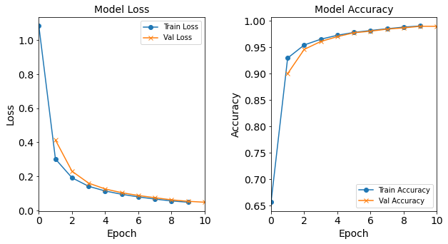
Figure: The model’s loss and accuracy as a function of epochs from the model 2H18N18N.
Exercises
Create additional code cells to run models (
3H18N18N18N).Solutions
def NN_Model_3H(hidden_neurons_1,hidden_neurons_2, hidden_neurons_3, learning_rate): """Definition of deep learning model with three dense hidden layers""" random_normal_init = tf.random_normal_initializer(mean=0.0, stddev=0.05) model = Sequential([ # More hidden layers can be added here Dense(hidden_neurons_1, activation='relu', input_shape=(19,), kernel_initializer=random_normal_init), # Hidden Layer Dense(hidden_neurons_2, activation='relu', kernel_initializer=random_normal_init), # Hidden Layer Dense(hidden_neurons_3, activation='relu', kernel_initializer=random_normal_init), # Hidden Layer Dense(18, activation='softmax', kernel_initializer=random_normal_init) # Output Layer ]) adam_opt = Adam(lr=learning_rate, beta_1=0.9, beta_2=0.999, amsgrad=False) model.compile(optimizer=adam_opt, loss='categorical_crossentropy', metrics=['accuracy']) return model"""Construct & train a NN_Model with 3 hidden layers, 18 neurons in each hidden layer"""; model_3H18N18N18N = NN_Model_3H(18,18,18,0.0003) model_3H18N18N18N_history = model_3H18N18N18N.fit(train_features, train_L_onehot, epochs=10, batch_size=32, validation_data=(test_features, test_L_onehot), verbose=2) saveOutputs_HL(3, model_3H18N18N18N_history, model_3H18N18N18N)Epoch 1/10 6827/6827 - 7s - loss: 1.1240 - accuracy: 0.6477 - val_loss: 0.5027 - val_accuracy: 0.8692 Epoch 2/10 6827/6827 - 7s - loss: 0.3834 - accuracy: 0.9127 - val_loss: 0.3083 - val_accuracy: 0.9344 Epoch 3/10 6827/6827 - 7s - loss: 0.2580 - accuracy: 0.9461 - val_loss: 0.2213 - val_accuracy: 0.9559 Epoch 4/10 6827/6827 - 7s - loss: 0.1900 - accuracy: 0.9584 - val_loss: 0.1637 - val_accuracy: 0.9624 Epoch 5/10 6827/6827 - 7s - loss: 0.1425 - accuracy: 0.9639 - val_loss: 0.1233 - val_accuracy: 0.9668 Epoch 6/10 6827/6827 - 7s - loss: 0.1106 - accuracy: 0.9724 - val_loss: 0.0990 - val_accuracy: 0.9750 Epoch 7/10 6827/6827 - 7s - loss: 0.0906 - accuracy: 0.9789 - val_loss: 0.0814 - val_accuracy: 0.9817 Epoch 8/10 6827/6827 - 7s - loss: 0.0775 - accuracy: 0.9823 - val_loss: 0.0737 - val_accuracy: 0.9838 Epoch 9/10 6827/6827 - 7s - loss: 0.0688 - accuracy: 0.9842 - val_loss: 0.0674 - val_accuracy: 0.9829 Epoch 10/10 6827/6827 - 7s - loss: 0.0622 - accuracy: 0.9857 - val_loss: 0.0594 - val_accuracy: 0.9842
Figure: The model’s loss and accuracy as a function of epochs from the model 3H18N18N18N.
For simplicity sake, we will just save the output from the baseline model again.
saveOutputs_HL(1, model_1H_history, model_1H)
Post-Processing: Varying Layers
This was executed similar to before. All of the graphs follow the usual trend and converge as expected.
# outer directory
dirPathHL = dir0_HL

# The hidden layers for each experiment/model.
# The number of hidden neurons in each layer input as a list.
# Each number in the list is the number of neurons in that layer.
listHL = [[18], [18, 18], [18, 18, 18]] # change this line to reflect the experiments you did run!

# Number of epochs - 1
lastEpochNum = 9

# Initalize. This will hold the list of dictionaries of last epoch metrics
# (loss, val_loss, accuracy, val_accuracy)
all_lastEpochMetrics_HL = []

# Fill in the rows for the DataFrame
for HL in listHL:
    # Read the history CSV file and get the last row's data, which corresponds to the last epoch data.
    result_csv = fn_out_history_XH(dirPathHL, HL, 0.0003, 32, lastEpochNum+1)
    print("Reading:", result_csv)
    epochMetrics = pd.read_csv(result_csv)
    # Fetch the loss, accuracy, val_loss, and val_accuracy from the last epoch
    # (should be the last row in the CSV file unless there's something wrong
    # during the traning)
    lastEpochMetrics = epochMetrics.iloc[lastEpochNum, :].to_dict()
    # Attach the "neurons" value
    lastEpochMetrics["neurons"] = HL
    all_lastEpochMetrics_HL.append(lastEpochMetrics)

df_HL = pd.DataFrame(all_lastEpochMetrics_HL,
                     columns=["neurons", "loss", "accuracy", "val_loss", "val_accuracy"])

print(df_HL)

df_HL.to_csv("post_processing_layers.csv", index=False)
        neurons      loss  accuracy  val_loss  val_accuracy
0          [18]  0.099545  0.978559  0.097021      0.979219
1      [18, 18]  0.047560  0.989797  0.047009      0.988996
2  [18, 18, 18]  0.062198  0.985700  0.059368      0.984199
CHALLENGE QUESTION
(Optional, challenging) Try to vary the number of neurons in the hidden layers (add / subtract as needed) and check the results.
Additional Tuning Opportunities
There are other hyperparameters that can be adjusted, including changing:
- Optimizer (try optimizers other than
Adam) - Activation function (this is actually a part of the network’s architecture)
- And many more!
We encourage you to explore the effects of changing these in your network.
Summary
Iterative model tuning - adjusting the model (i.e. set of hyperparameters) to achieve the best performance is an important and laborous process. By going through this notebook it will be obvious that creating a deep learning experiment using a jupyter notebook will get messy and laborious. By the end of this module, you will learn how to utilize scripting as well as using the power of HPC to alleviate the pain of executing block by block of jupyter notebook and make this experiment fast.
How was the experiment of model tuning so far? Frustrating? Confusing? So, let’s be honest, any machine learning experiment is going to have some level of uncertainty when dealing with unseen data. Especially when you don’t know how your model will respond to your features. This makes the model tuning process a messy process! In this notebook, by learning about different neural networks hyperparameters and tuning some of them, including hidden layers, hidden neurons, learning rate, etc., we tried to monitor the effects on accuracy. These accuracy results were also visualized graphically and saved to CSV format for later.
Post-analysis and take-aways from these experiments are located in a later lesson. The post-analysis takes the post-processing model output and metadata and utilizes plots to track how increasing or decreasing the value of one hyperparameter affects the model’s accuracy.
Now, shift your attention from the model tuning process to the platform in which we did our experiment. Jupyter notebook is an excellent platform to create code, experiment on and get the results. The single cell to single cell execution of commands seems tedious. In the beginning of this notebook, we introduced how doing experiments in this fashion is messy in jupyter notebook. So, I highly recommend to do such experiments with scripting.
In the next lesson, we will introduce how to convert an existing Jupyter notebook to a Python script that can be executed by HPC without constant interaction from the user. More importantly, we will learn how to launch experiments utilizing scripting!
Further Research:
Key Points
Neural network models are tuned by tweaking the architecture and tuning the training hyperparameters.
Some common hyperparameters to tune include the number of hidden layers (depth of the network), number of neurons in each hidden layer (width of the layer), learning rate (step rate), and batch size (number of training samples before updating).