Overview of Deep Neural Network Concepts
Overview
Teaching: 0 min
Exercises: 0 minQuestions
What is a neuron?
How does a neuron work?
What is a neural network?
How is a neural network trained?
Objectives
The basic components of a neural network.
The general idea of model construction.
From Neuron to Neural Networks
An artificial neural network (often just called a neural network) is inspired by the structure of our brain. The human brain is an object of wonder: It contains 86 billion neurons and over 100 trillion synapses (special connectors between neurons). It is capable of performing very high cognitive functions such as recognizing the objects that our eyes see, comprehending the sounds that our ears hear, reading, speaking, and even reasoning!
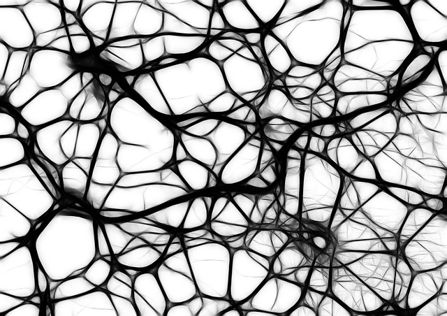
Figure: An artist’s rendition of a biological neural network (credit: Max Pixel)
In biology, a neuron contains one or more “input terminals” (dendrites is the biological term), and one “output terminal” (axon). Signals received from the dendrites will excite the neuron to produce an output signal. Not all inputs are equal in importance; some inputs may more strongly influence the neuron compared to others.
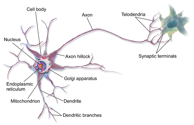
Figure: An illustration of a single neuron (credit: Wikipedia user BruceBlaus).
A neural network model, like any other machine learning models, is essentially a mathematical function with one or more inputs and one or more outputs. It comprises many artificial neurons that are interconnected in a particular way, with the goal of producing a correct set of responses upon receiving a set of inputs. Each neuron is essentially a mathematical object whose behavior is inspired by how biological neurons work. Neural networks can be used for a wide variety of classification tasks. For example, a properly trained convolutional neural network (a type of neural network specializing in image-related tasks) takes an image of a dog and classify the output as a dog (as opposed to a cow). In this case,
-
the input would be an array of pixel values of the picture, and
-
the output would be a very tall 1-D array with a value of “one” for the index belonging to the “dog” category, with zeros everywhere else.
There are also other neural network models which are trained for regression tasks, i.e., to simulate continuous mathematical functions.
Difference Between Biological and Artificial Neural Network
Despite their similarities, there are many interesting differences between biological neural systems and artificial neural network models. One key difference covers how they work under the hood: Biological neurons communicate, or transmit signals, using electrical impulses called action potentials, or often called spikes. Therefore, we speak of biological neurons as “firing” over time; the timing and frequency of the spikes carry information. In contrast, an artificial neural network takes in numerical values (in the form of one or more vectors or tensors), and produce numerical values (also a scalar, vector, or tensor). It does not send signals as “spikes” like its biological counterpart.
An artificial neural network is a much simpler system that can be trained to perform a prescribed task; in contrast, biological neural systems are highly complex systems that can learn and adapt over time.
A Mathematical Model for One Neuron: Input, Layer, Activation Function, Output
Here is a neuron model that is widely used in neural network applications. For illustrative purposes, let’s consider a neuron that takes three inputs \(i(1)\), \(i(2)\), \(i(3)\) and produces one output \(o(1)\). The three inputs and one output respectively form the input layer and output layer. Generally, a layer is the highest-level building block in deep learning. It is a container that usually has a set of elements either sending values to another layer or receiving values from another layer. The “wires” that connect the input signals to the neuron have different strength factors (usually called weights), i.e., \(w(1)\), \(w(2)\), \(w(3)\). Diagramatically, the neuron looks like this:
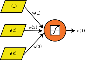
Figure: A 3 input single neuron model that omits the bias factor \(b\).
The inputs are combined in a linear fashion at the neuron input point:
\[z = w(1) i(1) + w(2) i(2) + w(3) i(3) + b .\]You may recognize that this is just a dot product plus a constant. (There is a bias factor \(b\) that is omitted in this illustration; but this does not compromise the point illustrated here.) The output is obtained by applying a nonlinear function called activation function, denoted by \(g(z)\), to this combined input. The nonlinearity of \(g(z)\) is the crucial feature of neurons that form a neural network: In classification, this nonlinearity allows the model to tease out the different classes separated by complicated boundaries in the feature space. (This blog article by Chris Olah offers some illustrative examples.) A classic choice for the nonlinear function is the sigmoid function:
\[g(z) = \frac{1}{1 + \exp(-z)} .\]This illustration shows the shape of the sigmoid function (where \(z\) is located at the horizontal axis):
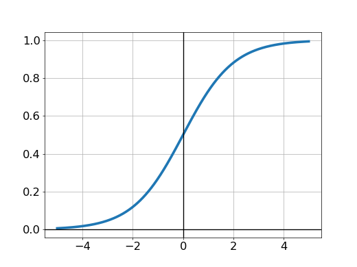
Figure: The shape of the sigmoid function \(g(z)\) where \(z\) is on the horizontal axis.
Activation Functions
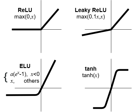
There are several other activation functions that are widely used in neural networks:
Figure: Several types of activation functions widely used in neural networks. For these diagrams, \(z\) is replaced with \(x\).
If the parameters \(w(1)...w(3)\) are known, then computing the input is as simple as using this one-line Python expression:
out = 1 / (1 + numpy.exp(-numpy.dot(w, i)))
In general mathematical terms, given the input vector \(\mathbf{i} = (i(1), i(2), i(3), ...)\) and weight vector \(\mathbf{w} = (w(1), w(2), w(3), ...)\), the output of the neuron is given by
\[o(\mathbf{i}) = g(\mathbf{w} \cdot \mathbf{i} + b).\]The output is the activation function, \(g(z)\), of the dot product of the weights and inputs plus the bias, \(b\).
Training the Neuron
How can we make this neuron predict the output \(o(1)\) given a set of inputs \(i(1)...i(3)\)? We need to train it according to some examples of inputs and outputs. Here, we follow a simple illustrative example (drawn from Medium articles by Milo Spencer-Harper and Andrew Trask). For simplicity, each of the inputs and outputs is binary (either one or zero). Here is an example of input sets and the expected corresponding outputs (“outcomes”).
| Case number | i(1) | i(2) | i(3) | o(1) |
|---|---|---|---|---|
| 1 | 0 | 0 | 1 | 0 |
| 2 | 1 | 1 | 1 | 1 |
| 3 | 1 | 0 | 1 | 1 |
| 4 | 0 | 1 | 1 | 0 |
Cases 1–4 above, with the known outputs, is collectively known as training data. The inputs are called features, and the outputs are called labels.
Here’s a machine learning question: What should the output be for the following input?
| Case number | i(1) | i(2) | i(3) | o(1) |
|---|---|---|---|---|
| 5 | 1 | 0 | 0 | ? |
Loss Function and Backpropagation
What happens in the training phase? In the example above, training simply involves an iterative procedure to adjust the weights (\(w(1)\), \(w(2)\) and \(w(3)\)). The goal for the training phase is to make the neuron mimic the behavior shown in the training data above as closely as possible, while being general enough to accurately predict the output for new cases.
The overall dataflow of the training phase is shown in the following figure:
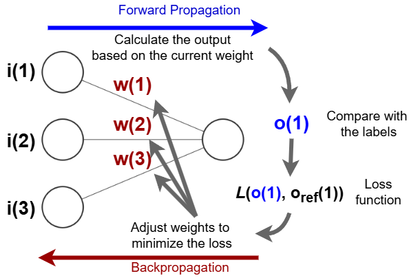
Figure: The overall dataflow of the training phase.
In general, the training phase of a neural network includes the following procedures:
-
Start with an initial guess for the network weights or parameters. (Sometimes, a guess from a similar kind of network that has been well-trained can be used, which will tremendously speed up the training process.)
-
Compute the predicted outcome (\(o(1)\) in the single-neuron case) for every training input. This is called forward propogation, which calculates the output of the neuron (or neural network) from a given set of inputs and the current state of model parameters (weights and biases).
-
Compute the discrepancy of the predicted outcome against the actual output of the training data (in this case, \(o_\mathrm{ref}(1)\)). This discrepancy is quantified by a loss function, which provides a collective measure of how far off the predictions are (i.e., for the single-neuron case, the \(o(1)\), for every sample) with respect to the expected outputs (the labels of training data). A large value of the loss function means a large discrepancy between the predicted and expected label values. In principle, the goal of the training phase is to minimize the loss function of the network.
-
Apply a correction procedure to update the weights so as to bring the predicted outcome closer to the expected outcome (the training label). For neural networks, an algorithm called backpropagation is used to compute the necessary corrections to the weights.
-
Repeat steps 2–4 until certain criteria are met (e.g., after \(N\) number of iterations or after the loss function falls below a certain threshold).
Since the topic of neural networks is quite extensive, we will not discuss in much detail technical matters such as the loss function (point 3 above), weight correction procedure (point 4), or convergence criteria (point 5). Interested readers are encouraged to pursue these matters on their own. The Python codes provided in the hands-on activities throughout this lesson should provide reasonable starting points.
Underfitting and Overfitting: Variance vs Bias
We mentioned earlier that losses are an inherent part of machine learning. Unless we have perfect data and the perfect model to describe the data, it is unlikely that we perfectly describe our data. The best model obtained via machine learning must strike a balance between two extremes: variance and bias. This balance is very important if we want our model to be generalizable to new cases, i.e., to input data not seen before.
-
Variance is defined as “an error [arising] from sensitivity to small fluctuations in the training dataset.” (Wikipedia) A model with high variance is overly sensitive to the fluctuations in the training dataset, usually because it has too much flexibility. In other words, it follows the behavior of the training data too closely, including the noise. This phenomenon is called overfitting. A model with high variance will not work well with new data: The useless information (noise) gets encoded into the model and ruins its generalizability.
An example of overfitting is shown in the following figure.
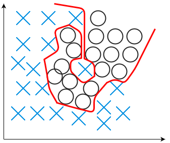
Figure: An example of overfitting.
-
Bias is the opposite extreme: “an error [arising] from erroneous assumptions in the learning algorithm.” (Wikipedia) A model with high bias is often not flexible enough to capture all the relevant features found in the data. Such a model, while having low variance (i.e., not changing much amidst data fluctuations), is also unable to give a good prediction because it misses the relevant relationship between features (input) and target outputs. This phenomenon is called underfitting.
An example of underfitting is shown as follows.
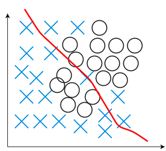
Figure: An example of underfitting.
Either of these extremes will prevent the model from giving a good prediction.
Inference (Prediction)
After a network is trained, it is ready to be used to perform its job
(such as recognizing images, differentiating between good and harmful
network traffic, etc.).
This process is often called inference.
Compared to training, inference is computationally much cheaper.
The overall diagram for inference is shown in the following figure:
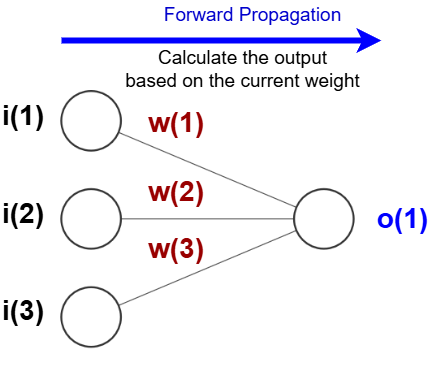
Figure: The overall dataflow of the inference phase.
Deep(er) Neural Network: Putting More Neurons Together
There is not much that a single neuron can do. One obvious limitation is that a single neuron can only produce a binary prediction (i.e., a “yes” or a “no”). Much greater prediction power is obtained by constructing a network of neurons. Here is an example illustration of how one can construct a network comprising many neurons:

Figure: An illustration of a simple neural network with one hidden layer (credit: Glosser.ca, with modification).
This is called a fully connected dense network. The network in this illustration has three layers:
-
the input layer, colored yellow;
-
one hidden layer, colored green;
-
the output layer, colored orange-red.
The input layer does not perform any computation; hence, this network really has only two neuron layers, consisting of a total of six neurons (four in the hidden layer plus two in the output layer). Neuron layers are those that have the “thinking” capability in the network. In the fully connected dense network, each neuron from a layer is connected to all the neurons in the subsequent layer.
A neural network is considered “deep” if it has many hidden layers. The exact definition of “deep” varies by practitioners; but generally, such a network has two or more hidden layers. Deep networks provide the necessary flexibility for the network to be “molded” according to the training data. Deep learning refers to the utilization of such a deep network for machine learning modeling.
Steps for Deep Learning
The steps involved in deep learning are very similar to the steps of traditional machine learning:
-
Loading and preprocessing the input data;
-
Defining a neural network model;
-
Compiling the network (model);
-
Fitting (training) the network using the training data;
-
Evaluating the performance of the network;
-
Improving the model’s performance iteratively by adjusting the network’s hyperparameters and retraining;
-
Deploying the model to make predictions (i.e., “inference”).
The training flow described earlier for one neuron can be applied to deep neural networks. These steps will be explained in more depth in a later episode.
Hardware Acceleration for Deep Neural Networks
The process of training is computationally very intensive, as we will experience in this workshop. For this reason, people often use highly parallel computing hardware such as supercomputers or graphics processing units (GPUs).
Key Points
Deep neural networks have linear and nonlinear parts.
Activation functions add the nonlinear component to the model.
Forward propagation calculates the output based on the current parameters.
Backpropagation is used to adjust the network parameters.
An HPC can be adopted to speed up the training and inference processes.