Dealing with Issues in Data and Model Training
Overview
Teaching: 20 min
Exercises: 40 minQuestions
What are common data issues in Machine Learning (ML)?
How do data issues impact ML model performance?
How to identify data issue effects on ML model performance?
How to address these data issues?
How to identify issues in ML model training caused by overfitting and underfitting?
How to address overfitting and underfitting?
Objectives
Understand common data issues and their effects.
Learn metrics for evaluating model performance.
Identify and diagnose the effects of data issues.
Explore methods to address data issues.
Recognize underfitting and overfitting in ML.
Learn approaches to mitigate overfitting and underfitting.
Introduction
In the previous episodes, we trained and validated NN models assuming that the dataset is ideal for the purpose of training the models. We also assumed that the training algorithm works flawlessly to produce a well-performing models. In real world, these two things do not always hold true. This lesson episode introduces methods to address issues related to dataset and model training; they are intended to produce a reliable model for real-world deployment.
Real-world datasets often contain imperfections such as missing values, inaccurate labels, imbalance among classes, and many other issues. When such datasets are used to train and validate machine learning models, these issues can negatively affect the model’s performance. Understanding, detecting and mitigating these data issues are essential for ensuring that the trained models perform effectively in real-world applications.
In training a machine learning model, one must be cautious of issues such as overfitting, underfitting, or gradient problems. These training-related problems also lead to degradation in model’s performance and reliability. We will show how we can identify and address issues related to model training.
We will continue to use the smartphone app classification task
with sherlock_18apps dataset to illustrate the dataset-related problems.
In previous episodes,
we built and tuned neural network models with Keras,
and we were able to achieve accuracy which appears to be impressive
(over 99%).
However, as we shall see in this episode,
there is more to it than a single-valued accuracy metric
if we aim to build a well-balanced classifier.
We will need to use other metrics that can
capture a model’s performance in greater details,
and use them to guide improvements in our modeling.
Along the way, we will answer following questions:
- What are the common data and training issues in ML?
- How do these issues affect model performance?
- What other metircs can help us to detect these issues?
- What techniques can we use to mitigate these issues to improve the model’s overall performance?
Common Data Issues and Their Impacts
Here are five common data issues:
Missing Values
One common issue in real-world datasets is missing values, which occur when certain pieces of data are simply absent—like questions left unanswered on a survey. This can happen for various reasons, such as hardware malfunctions, software errors, human oversight, or incomplete data collection. For example, in a fitness tracking app, heart rate data might be missing during periods when the wearable device loses contact with the skin, or the device runs out of battery, or the Bluetooth connection with the phone is temporarily interrupted.
Missing values can pose serious problems during model training.
Many machine learning models, including NN models,
would fail completely if they encounter missing values,
which are encoded as NaN (short for Not a Number).
Even when training continues,
missing data can reduce the amount of usable information,
or lead to biased predictions if not handled carefully.
Class Imbalance
In many real-world datasets, some classes may have significantly more samples than the others; this situation is known as class imbalance. The following graph shows the number of images (samples) in a dataset that may be used to train image classification models:
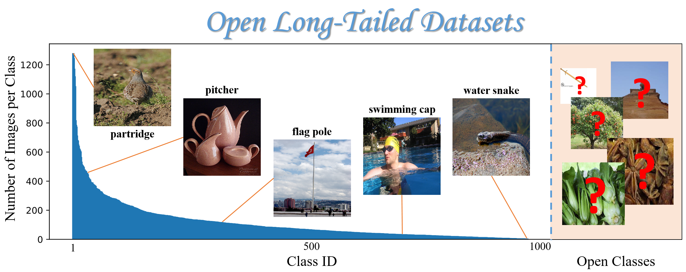
Open Long Tailed Datasets. Curated by Z. Liu, Z. Miao, X. Zhan, J. Wang, B. Gong, & S.X. Yu (2019). Published in this paper: “Large-Scale Long-Tailed Recognition in an Open World”. In Proceedings of the IEEE/CVF Conference on Computer Vision and Pattern Recognition, pp. 2537-2546.
In this dataset, there are over 1200 samples for partridge (a kind of bird), whereas there are fewer than 20 samples for water snake. In general, there are a few common scenarios which lead to class imbalance in a dataset:
-
Rare events: Certain events naturally occur far less frequently than others. In fraud detection, for example, only a tiny fraction of transactions are fraudulent — often less than 0.1%. In computer networking, cyber attack events are also extremely rare and difficult spot among the vast number of benign network packets. Similarly, rare diseases such as certain types of cancer or genetic disorders may affect only a small fraction of the population (e.g., 1 in 100,000 individuals). These naturally low-frequency events lead to class imbalance, where one class significantly outnumbers another.
-
Long-tail distribution: In many domains, data follows a long-tail distribution, where a few classes (the “head”) have a large number of samples, while many other classes (the “tail”) have very few samples. This pheonemnon is shown in the Open Long Tailed Datasets graph shown earlier.
-
Data collection bias: During data collection, certain categories of samples may be overrepresented or underrepresented due to imperfect sampling methods, limitations of tools, or human factors, resulting in an imbalanced dataset.
More Real-World Class Imbalance
Can you think of more examples in real life where data is naturally imbalanced? Try to classify whether they are due to rare events, long-tail distribution, or data collection bias. Discuss with your peers and share your ideas.
Hint: Try to come up with examples from different domains like social media, education, or transportation.
Examples
- In social media platforms, the number of likes or followers per user is highly imbalanced — a few users have millions, while most have only a few.
- In education platforms, only a small percentage of students might drop out of a course, making “dropout” cases rare.
- In transportation, vehicle breakdowns are much less frequent compared to normal trips, creating an imbalance in incident reports.
- In industrial equipment monitoring, failures are infrequent compared to normal operations.
Class imbalance can pose serious challenges for machine learning models. When training a classification model with an imbalanced dataset where most samples belong to one class, the model tends to overly focus on that majority class and overlook the minority ones. This leads to poor performance in classifying the minority classes. This problem is often masked when we use the overall model accuracy as a metric during model training, since it can be artificially high due its correct predictions for the dominant class. We will need to use other metrics that are more sensitive to minority classes, such as precision, recall, and F1-score.
Inaccurate Data
Another common issue in real-world datasets is inaccurate data, which refers to values that are recorded incorrectly, mislabeled, or corrupted. These inaccuracies can occur due to human errors (whether intentional or not), sensor glitches, miscommunication in labeling processes, or even software bugs.
For instance, in a smartphone app usage dataset, an app might be misclassified as a game when it’s actually a productivity tool. Similarly, sensor readings from a wearable device could contain spikes or flat lines due to poor contact or temporary hardware issues.
Inaccurate data can mislead the model during training by providing incorrect patterns to learn from. Unlike missing data, inaccuracies are harder to detect automatically—they may look like valid data but theay are actually wrong. This makes data cleaning and validation steps critical before training a model.
Outliers
Outliers are data points that deviate significantly from the rest of the dataset. They may occur due to genuine rare events. Suppose a smartwatch or fitness tracker measures 100,000 steps of walk in a day, whereas it typically registers under 10,000 steps per day. This measurement might be valid in very rare cases (e.g., for an extreme athlete during his/her competition day). Outlier values must be carefully examined to rule out the possibility of errors in data. For example, in the case of fitness tracker word by common people, an outlier measurement of 100,000 steps in a day is most likely due to an error.
Outliers can distort training, especially in models sensitive to numerical scales like linear regression or neural networks. They may cause the model to place undue emphasis on extreme cases, which can shift decision boundaries in unhelpful ways. In classification tasks, a single mislabeled or extreme-value point can disproportionately affect the learned model, particularly if the dataset is small.
Irrelevant Features
Not all features in a dataset contribute meaningfully to the task at hand. Irrelevant features are features that have little or no predictive power for the target label, but are still included in the data. These may come from overly broad data collection, automatic logging, or simply poor feature selection.
For example, in our smartphone app classification task, a user’s phone wallpaper color or device serial number is unlikely to help predict type of app being used. These features may introduce noise, confuse the model, where the model learns patterns that are specific to the training set but do not generalize to real-world data.
The presence of irrelevant features increases the dimensionality of the input, which can slow down training, increase memory usage, and even worsen the model’s performance due to the curse of dimensionality the phenomenon where the high-dimensionality of the data makes it harder for models to learn meaningful patterns.
Real-World Data Issues
For each of the five data issues discussed above, can you think of more real-world examples from different domains? Try to think about how each data issue might appear in our smartphone app classification scenario. Discuss your thoughts with your peers.
Examples
- Missing Values
- Different domain: In healthcare, patient records may have missing blood pressure readings due to skipped checkups or broken devices.
- Smartphone App: A fitness app may lose heart rate or step count data when the wearable device disconnects.
- Class Imbalance
- Different domain: In fraud detection, fraudulent transactions make up less than 1% of all transactions.
- Smartphone App: Most apps belong to popular categories like “Social” or “Entertainment”, while categories like “Accessibility” are rare.
- Inaccurate Data
- Different domain: In financial systems, a stock trade might be recorded with the wrong timestamp or price due to system errors.
- Smartphone App: An app used for reading the news might be mislabeled as a “Game” during data annotation.
- Irrelevant Features
- Different domain: In education, a student’s favorite color may be included in the data but is irrelevant to predicting course success.
- Smartphone App: The user’s device wallpaper or battery level is unlikely to help predict app type.
- Outliers
- Different domain: A person recording 10,000 calories in a diet app in one day might be an entry mistake or an extreme case.
- Smartphone App: A user opening an app 500 times in one day is an unusual usage pattern that may distort training.
Hands-On Activity: Exploring Data Issues in sherlock_18apps
The sherlock_18apps dataset, which we’ve been using for smartphone app classification,
is sourced from real-world, authentically collected data.
Therefore, it may contain imperfections that can impact model performance.
In this hands-on activity, you’ll explore the sherlock_18apps dataset to identify potential data issues.
This exploration will help you connect the theoretical data issues discussed earlier to practical observations,
leading to a better understanding.
Loading Required Python Libraries and Objects
Ensure the following libraries are loaded in your environment:
import os
import sys
import pandas as pd
import numpy as np
import matplotlib.pyplot as plt
import matplotlib.gridspec as gridspec
import sklearn
from sklearn import preprocessing
from sklearn.model_selection import train_test_split
from sklearn.metrics import accuracy_score, confusion_matrix, classification_report
import tensorflow as tf
import tensorflow.keras as keras
from tensorflow.keras.models import Sequential, load_model
from tensorflow.keras.layers import Dense
from tensorflow.keras.optimizers import Adam
Exploring Data Issues in
sherlock_18appsDatasetIn this activity, we focus on missing values and class imbalance in the
sherlock_18appsdataset because they are the most straightforward issues to identify by examining data and class distributions.Load and check the
sherlock_18appsdataset usingsherlock_ML_toolboxand answer:
- Which features have missing values, and how many?
- Are classes in the dataset imbalanced?
Solution
1. Inspecting Missing Values:
Import the function
load_prep_data_18appsfromsherlock_ML_toolboxto load dataset.from sherlock_ML_toolbox import load_prep_data_18appsLoad the dataset using
load_prep_data_18appsto check for missing values.datafile = "sherlock/sherlock_18apps.csv" df, df2, labels, df_labels_onehot, df_features = load_prep_data_18apps(datafile,print_summary=False)Output:
Loading input data from: sherlock/sherlock_18apps.csv
Cleaning:
- dropped 2 columns:  ['cminflt', 'guest_time']
- remaining missing data (per feature):
CPU_USAGE      52
cutime         52
num_threads    52
priority       52
rss            52
state          52
stime          52
utime          52
vsize          52
dtype: int64
- dropping the rest of missing data
- remaining shape: (273077, 17)
Step: Separating the labels (ApplicationName) from the features.
Step: Converting all non-numerical features to one-hot encoding.
Step: Feature scaling with StandardScaler
Analysis: The output shows that the
sherlock_18appsdataset has missing values in multiple features: CPU_USAGE, cutime, num_threads, priority, rss, state, stime, utime, and vsize, each with 52 missing entries.
2. Inspecting Class Imbalance:
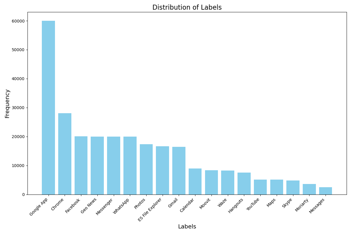
To investigate whether there is a class imbalance issue in the dataset, we define a function to print and visualize the label distribution.
def visualize_label_distribution(labels):
    """
    Visualize the distribution of labels and print the frequency distribution.

    Parameters:
    labels (pd.Series): A pandas Series containing the labels (e.g., ApplicationName).
    """
    # Check the frequency distribution of each category
    labels_distribution = labels.value_counts()

    # Print the frequency distribution
    print("Frequency Distribution of Labels:")
    print(labels_distribution)

    # Set the figure size
    plt.figure(figsize=(12, 8))

    # Create a bar plot
    plt.bar(labels_distribution.index, labels_distribution.values, color='skyblue')

    # Add title and labels
    plt.title('Distribution of Labels', fontsize=16)
    plt.xlabel('Labels', fontsize=14)
    plt.ylabel('Frequency', fontsize=14)

    # Rotate x-axis labels for better readability
    plt.xticks(rotation=45, ha='right')

    # Display the plot
    plt.tight_layout()
    plt.show()
Apply the function to the variable
labels, which is derived from the output ofload_prep_data_18apps.visualize_label_distribution(labels)Output:
Frequency Distribution of Labels:
Google App          60001
Chrome             28045
Facebook           20103
Geo News          19991
Messenger         19989
WhatsApp          19985
Photos            17380
ES File Explorer  16660
Gmail             16414
Calendar           8986
Moovit            8365
Waze              8228
Hangouts          7601
YouTube           5173
Maps              5157
Skype             4876
Moriarty          3616
Messages          2507
Name: ApplicationName, dtype: int64
Analysis: The output reveals a significant class imbalance in the
sherlock_18appsdataset. The Google App is heavily over-represented with 60,001 samples, while apps like Messages (2,507 samples), Moriarty (3,616 samples), and Skype (4,876 samples) are under-represented.Conclusion:
By exploring and answeing above two questions, we confirm the presence of both missing values and class imbalance in the
sherlock_18appsdataset.
Common Model Training Issues and Their Impacts
Training a machine learning (ML) model involves optimizing its parameters to learn patterns from data. Ideally, the model’s complexity will align with the data’s complexity, allowing it to learn general patterns effectively and form a decision boundary that accurately separates different classes of samples, performing well on both training and validation sets.
However, when the model’s complexity does not align with the data’s complexity,
training problems such as overfitting and underfitting arise,
leading to poor performance or unstable training.
These issues can prevent models from generalizing effectively in tasks like sherlock_18apps classification.
Understanding and addressing these training issues is crucial for building reliable ML models.
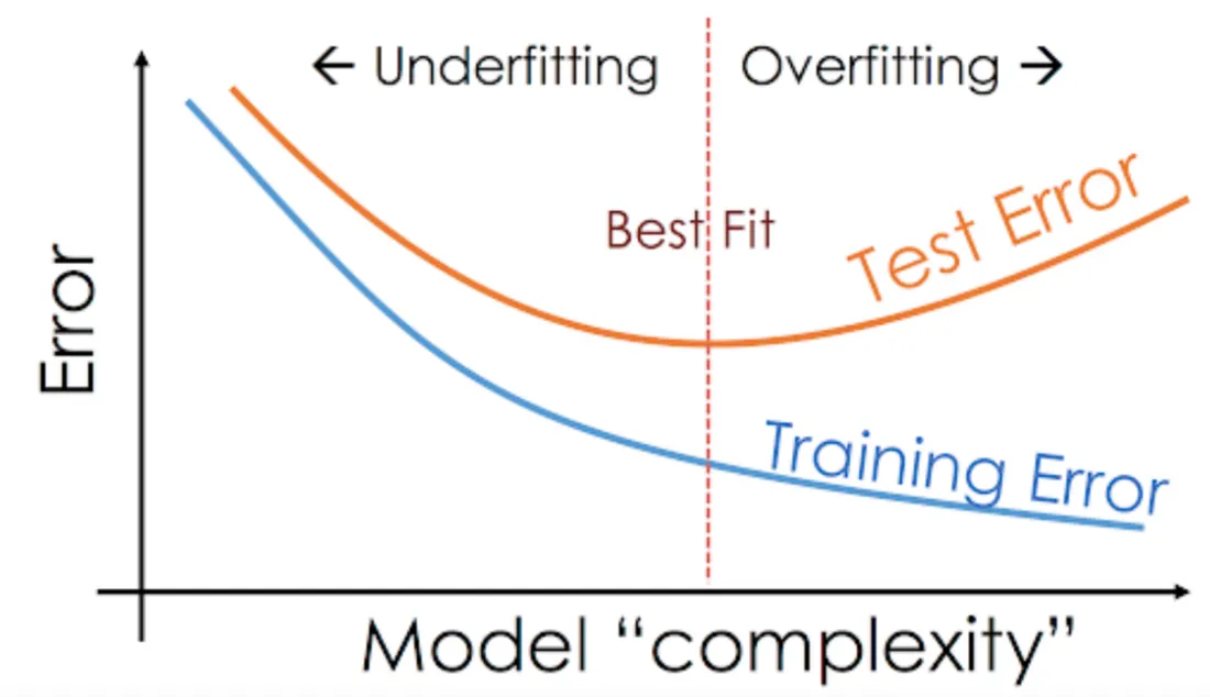
Overfitting
Overfitting occurs when a machine learning model becomes overly attuned to the noise and specific details of the training data, failing to capture generalizable patterns that apply to new, unseen data. A classic example is a student who memorizes every detail of practice questions, including irrelevant typos, and consequently fails to solve new problems that require genuine understanding.
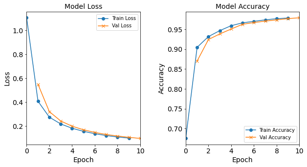
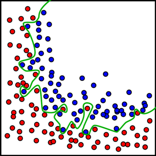
This issue is often reflected in the divergence between training and validation metrics: while the model achieves extremely low training loss and high training accuracy (sometimes approaching perfection), its performance on the validation set deteriorates significantly, with rising loss and dropping accuracy. This gap signals that the model has memorized the training data’s idiosyncrasies rather than learning underlying trends, a critical flaw for real-world applications where data variability is inevitable.
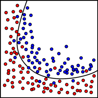
Visually, overfitting can be understood through the lens of decision boundaries in simplified feature spaces. In a two-dimensional example, an overfitted model might produce a highly complex, “wiggly” decision boundary that tightly wraps around every training point, even those influenced by random noise. Unlike a smooth, generalized boundary that captures the core separation between classes, this overly intricate boundary reflects the model’s attempt to explain every nuance of the training data—including irrelevant or misleading details. The result is a model that performs flawlessly on the training set but struggles to classify new samples correctly, as shown in the side-by-side illustrations below.

Underfitting
Underfitting occurs when a machine learning model is too simple relative to the data’s complexity, failing to capture the underlying patterns. This typically happens when the model has insufficient complexity (e.g., too few layers or parameters) or is not trained long enough to learn meaningful trends in the data. A typical example is a weather app that uses only temperature to predict rain, ignoring important factors like humidity and pressure. Such a model will fail to produce accurate forecasts because it lacks the capacity to understand the true complexity of the problem.
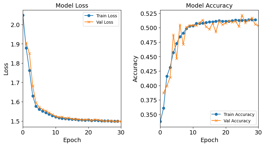
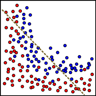
This issue is often reflected in the convergence of training and validation metrics at suboptimal levels: the model exhibits high training loss and low training accuracy, with similar poor performance on the validation set. This lack of divergence between training and validation metrics signals that the model has not learned meaningful trends from the training data, rendering it ineffective for real-world applications where capturing essential patterns is crucial.
Visually, underfitting can be understood through the lens of decision boundaries in simplified feature spaces. In a two-dimensional example, an underfitted model might produce an overly simplistic decision boundary, such as a straight line, that fails to adequately separate the classes, leaving many points misclassified. Unlike a well-balanced boundary that captures the core separation between classes, this rudimentary boundary reflects the model’s inability to model the data’s complexity. The result is a model that performs poorly on both training and validation sets, as shown in the side-by-side illustrations below.
Alternative Evaluation Metrics for Model Performance
In previous episodes, we primarily used accuracy to evaluate ML model performance.
While intuitive, accuracy can be misleading in imbalanced datasets.
A model might achieve high overall accuracy by correctly predicting majority classes
while failing on minority classes.
For example, the baseline model we developed in previous episodes for sherlock_18apps
reports a high overall accuracy, even with the dataset’s significant imbalance.
However, we don’t know whether the model performs well across all classes,
particularly for minority classes.
In this section, we will introduce several commonly used evaluation metrics beyond accuracy,
including precision, recall and F1 Score,
to comprehensively assess the performance of ML models,
even when dealing with imbalanced datasets where accuracy alone can be misleading.
We will apply these metrics to assess the true performance of sherlock_18apps classifier,
where the dataset shows a significant imbalance for minority classes.
Before diving into new metrics such as precision, recall and F1 Score, it is essential to first understand a foundational tool for evaluating the performance of a classification model: the confusion matrix, which provides a detailed and comprehensive breakdown of a classifier’s performance.
Confusion Matrix
A confusion matrix is a table that displays the detailed performance of a classification model on a set of test data where the true class values are known.
Let us begin with a binary classification problem, where there are only two possible classes, typically labeled as “Positive” and “Negative”. (The use of these terms comes from the common use cases for binary classification, where a positive class indicates the presence of a spam email, a cyber compromise, a malware, a threat, or a disease; whereas a negative class indicates the absence of those things, i.e. a safe, secure, or healthy condition.) Comparing the model’s predictions with the ground truths, there are four possible scenarios:
-
True Positive (TP): the model correctly classifies, or predicts, positive cases as positive.
-
True Negative (TN): The model correctly classifies negative cases as negative.
-
False Positive (FP): The model misclassifies (incorrectly predicts) negative cases as positive. This is also known as a false alarm. In this case, the ground truth is be negative, but the model prediction is positive.
-
False Negatives (FN): The model misclassifies positive cases as negative. This is also known as a miss.
In practice, these symbols (TP, TN, FP, FN) refer to the number of cases predicted by the model in the four scenarios mentioned above. The binary classification confusion matrix takes the form of a 2x2 table, or matrix:
| | Actual Class: Positive | Actual Class: Negative |
| :—————— | :————————- | :————————- |
| Predicted Class: Positive | True Positives (TP) | False Positives (FP) |
| Predicted Class: Negative | False Negatives (FN) | True Negatives (TN) |
In DeapSECURE module 4: Deep Learning (Neural Network), we build and train a simple Neural Network model for a binary classification task using the preprocessed sherlock_2apps dataset in the episode “An Introduction to Keras with Binary Classification Task”: distinguishing between two smartphone applications, where the positive class is Facebook and the negative class is WhatsApp.
Suppose, after training our model, the confusion matrix obtained from the test dataset is as follows:
| Actual Class: Facebook (Positive) | Actual Class: WhatsApp (Negative) | |
|---|---|---|
| Predicted Class: Facebook (Positive) | 73817 (TP) | 2003 (FP) |
| Predicted Class: WhatsApp (Negative) | 16525 (FN) | 30078 (TN) |
Specifically:
- True Positives (TP) = 73817:
- This means the model correctly predicted 73,817 Facebook instances as Facebook. These are the correctly identified uses of the Facebook app.
- False Positives (FP) = 2003:
- This means the model incorrectly predicted 2,003 WhatsApp instances as Facebook. In other words, the model mistakenly identified 2,003 instances of WhatsApp usage as Facebook usage (a “false alarm”).
- False Negatives (FN) = 16525:
- This means the model incorrectly predicted 16,525 Facebook instances as WhatsApp. That is, the model failed to identify 16,525 instances of Facebook usage, mistaking them for WhatsApp (a “miss”).
- True Negatives (TN) = 30078:
- This means the model correctly predicted 30,078 WhatsApp instances as WhatsApp. These are the correctly identified uses of the WhatsApp app.
Through this example, we can clearly see how the model performed in distinguishing between Facebook and WhatsApp. Although the model identified a large number of True Positives (Facebook) and True Negatives (WhatsApp), there are still a certain number of false positives and false negatives, which are crucial areas to focus on when evaluating model performance.
However, in real-world scenarios, multi-class classification problems are far more prevalent.
While the core concepts of “true” and “false” predictions still apply,
a confusion matrix for multi-class classification expands to an N * N table,
where N is the number of classes.
Each row represents the instances in an actual class,
and each column represents the instances in a predicted class.
The element at (i, j) in the matrix indicates the number of instances that
actually belong to class i but were predicted by the model to belong to class j.
-
Diagonal elements (where
i = j): These represent the correct predictions for each class. For example, the value at(Class A, Class A)shows how many instances of Class A were correctly predicted as Class A. -
Off-diagonal elements (where
i ≠ j): These represent the misclassifications. The value at(Class A, Class B)means instances of Class A were incorrectly predicted as Class B.
Understanding this structure is crucial because it allows us to identify not only if a class is being misclassified, but also which other classes it is being confused with. With the confusion matrix, we no longer just look at overall accuracy. Instead, we can clearly see the types of errors our model makes when identifying each class of samples.
Challenge: Print Confusion Matrix for the Baseline Model
In the previous episode (e.g.,
24-keras-classify.md), we trained a baseline model forsherlock_18appsand printed its overall accuracy on the validation set.def NN_Model_1H(hidden_neurons, learning_rate): """Definition of deep learning model with one dense hidden layer""" model = Sequential([ # More hidden layers can be added here Dense(hidden_neurons, activation='relu', input_shape=(19,), kernel_initializer='random_normal'), # Hidden Layer Dense(18, activation='softmax', kernel_initializer='random_normal') # Output Layer ]) adam_opt = Adam(lr=learning_rate, beta_1=0.9, beta_2=0.999, amsgrad=False) model.compile(optimizer=adam_opt, loss='categorical_crossentropy', metrics=['accuracy']) return model model_1H = NN_Model_1H(18,0.0003) model_1H_history = model_1H.fit(train_features, train_L_onehot, epochs=10, batch_size=32, validation_data=(val_features, val_L_onehot), verbose=2)Epoch 1/10 6827/6827 - 7s - loss: 1.1037 - accuracy: 0.6752 - val_loss: 0.5488 - val_accuracy: 0.8702 Epoch 2/10 6827/6827 - 6s - loss: 0.4071 - accuracy: 0.9047 - val_loss: 0.3205 - val_accuracy: 0.9245 Epoch 3/10 6827/6827 - 6s - loss: 0.2743 - accuracy: 0.9319 - val_loss: 0.2425 - val_accuracy: 0.9385 Epoch 4/10 6827/6827 - 6s - loss: 0.2177 - accuracy: 0.9468 - val_loss: 0.1990 - val_accuracy: 0.9509 Epoch 5/10 6827/6827 - 6s - loss: 0.1818 - accuracy: 0.9592 - val_loss: 0.1692 - val_accuracy: 0.9628 Epoch 6/10 6827/6827 - 6s - loss: 0.1561 - accuracy: 0.9664 - val_loss: 0.1470 - val_accuracy: 0.9671 Epoch 7/10 6827/6827 - 6s - loss: 0.1363 - accuracy: 0.9703 - val_loss: 0.1296 - val_accuracy: 0.9708 Epoch 8/10 6827/6827 - 6s - loss: 0.1209 - accuracy: 0.9740 - val_loss: 0.1171 - val_accuracy: 0.9739 Epoch 9/10 6827/6827 - 6s - loss: 0.1089 - accuracy: 0.9769 - val_loss: 0.1058 - val_accuracy: 0.9770 Epoch 10/10 6827/6827 - 6s - loss: 0.0995 - accuracy: 0.9786 - val_loss: 0.0970 - val_accuracy: 0.9792This code gives us a single accuracy score, but it doesn’t show whether the class imbalance issue affect model’s performance, especially on minority classes.
Can you print the confusion matrix (like below showed Reference Confusion Matrix) to show the count of correct and incorrect predictions compared to the actual outcomes?
Reference Confusion Matrix (from episode
24-keras-classify.md, decision tree classifier):1829 1 0 0 0 0 0 0 0 0 0 18 0 0 0 0 1 0 0 5477 0 0 0 69 0 0 0 0 0 0 0 5 0 0 2 0 1 610 2753 0 0 25 0 5 0 1 1 1 0 2 0 0 0 0 0 0 0 4029 0 0 15 0 0 0 0 0 0 0 0 0 0 10 0 0 0 0 4006 0 0 0 0 0 0 0 0 0 0 0 0 0 64 28 0 0 0 3183 1 0 0 0 0 1 0 49 0 0 0 0 0 143 0 0 0 2 10459 0 0 0 15 0 0 0 0 0 1369 0 0 58 0 0 0 24 4 1408 0 1 0 0 0 1 0 0 11 0 3 39 0 0 0 0 1 0 935 0 0 0 0 0 1 0 4 0 0 0 0 0 0 0 0 0 1 486 0 0 0 8 0 0 0 0 0 0 0 0 0 0 0 0 0 0 4016 0 0 0 0 0 0 0 0 0 0 0 0 0 0 0 0 0 0 1697 0 0 0 0 0 0 0 13 0 0 4 0 0 0 0 0 0 0 680 1 0 0 0 0 0 0 0 0 0 0 0 0 0 0 0 6 0 3473 0 0 0 0 0 0 0 0 0 0 0 0 0 0 0 0 0 0 1003 0 0 0 0 0 0 0 3 0 0 0 0 0 0 0 0 0 0 1642 0 0 0 4 0 0 0 0 4 0 0 0 0 0 0 0 0 0 3897 0 0 0 0 0 0 116 0 0 0 0 0 0 0 0 0 0 0 897Solution
Firstly, we need to split the dataset and preprocess the data by importing the function
split_data_18appsfromsherlock_ML_toolbox.from sherlock_ML_toolbox import split_data_18apps train_features, val_features, train_labels, val_labels, train_L_onehot, val_L_onehot = split_data_18apps(df_features, labels, df_labels_onehot)Then, we train the baseline model.
model_1H = NN_Model_1H(18,0.0003)
model_1H_history = model_1H.fit(train_features,
 train_L_onehot,
 epochs=10, batch_size=32,
 validation_data=(val_features, val_L_onehot),
 verbose=2)
To output the confusion matrix, we need to define a new model evaluation function.
def model_evaluate_custom(model, test_F, test_L_one_hot):
    # 1. Get model predictions
    test_L_pred_prob = model.predict(test_F)
    test_L_pred_indices = np.argmax(test_L_pred_prob, axis=1)  # Predicted class indices

    # 2. Convert true one-hot encoded labels to class indices
    if isinstance(test_L_one_hot, pd.DataFrame):
        test_L_true_values = test_L_one_hot.values
    else:  # Assuming NumPy array
        test_L_true_values = test_L_one_hot

    test_L_true_indices = np.argmax(test_L_true_values, axis=1)  # True class indices

    num_classes = test_L_true_values.shape[1] # Get number of classes from the shape of the labels

    # 3. Calculate Confusion Matrix
    # The 'labels' parameter ensures the confusion matrix dimensions are consistent
    # with the number of classes (0 to num_classes-1)
    cm_labels = np.arange(num_classes)
    cm = confusion_matrix(test_L_true_indices, test_L_pred_indices, labels=cm_labels)

    return cm
Then we use the new model evaluation function to evaluate the trained baseline model, and print the confusion matrix.
conf_matrix = model_evaluate_custom(model_1H, val_features, val_L_onehot)
print("Confusion Matrix:")
print(conf_matrix)
Output:
Confusion Matrix:
[[ 1746     0     1     0     2    90     1     0     2     0     0     5     0     0     1     0     1     0]
 [    0  5199    36     0    33     1     0     1     4    25     0     0     0     1     0   250     3     0]
 [    2    21  3342     0     0     7     0     4     0     0     0     0     0    10     5     0     3     5]
 [    0     0     1  4017     0     1    22     6     0     0     4     1     0     0     0     0     0     2]
 [    0     0     0     0  4000     0     0     0     0     6     0     0     0     0     0     0     0     0]
 [   82     1    10     0     0  3198    21     2     5     0     0     0     0     1     2     0     1     3]
 [    4     1     1    34     0     3 11922     5     2     0    16     0     0     0     0     0     0     0]
 [    0     4     2     1     0    22     3  1464     0     0     0     0     0     0     0     9     2     0]
 [   11     2    11     0     0     0     0     0   951     0     0     0     0     2     4     0     1     1]
 [    0     2     0     0     2     0     0     0     0   474     0     0     0    16     0     1     0     0]
 [    0     0     1     0     0     0     1     0     0     0  4013     0     0     0     0     0     0     1]
 [    1     0     0     0     0     0     0     0     0     0     0  1695     0     0     0     0     1     0]
 [    0     1     0     0     4     0     0     1     0     0     0     0   692     0     0     0     0     0]
 [    9    18   198     0     0     0     1     0     2     0     0     0     0  3231    19     0     1     0]
 [    0     0     8     0     0     0     0     0     4     0     0     0     0     0   991     0     0     0]
 [    0     5     0     0     0     0     0     0     0     0     0     0     0     0     0  1637     3     0]
 [    0     1     0     0     0     0     0     0     2     0     0     0     0     0     0     0  3902     0]
 [    0     2     4     0     0     0     0     0     0     0     0     0     0     0     0     0     0  1007]]
Introducing Precision, Recall, and F1-Score
Indeed, the confusion matrix clearly displays the classification results, detailing the model’s predictions for each category. However, merely looking at these raw counts makes it difficult to intuitively judge whether the model’s performance on different classes is good or bad, especially when dealing with imbalanced datasets. To gain a deeper understanding of the model’s strengths and weaknesses, we need to convert these numbers into more insightful evaluation metrics. Here, we three crucial alternative evaluation metrics: precision, recall, and the F1-score. These metrics provide a more granular view of classification performance beyond just correct versus incorrect predictions.
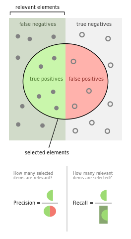
Precision
Definition: Precision measures how many of the samples predicted as a certain class actually belong to that class. It answers the question: “Of all the instances I predicted as positive, how many were actually positive?”
Formula:
Where:
-
TP (True Positive): The number of correctly predicted positive samples.
-
FP (False Positive): The number of samples incorrectly predicted as positive.
Intuitive Explanation:
Precision can be understood as “how reliable the model’s positive predictions are.”
For example, if your model predicts 100 apps as “Moriarty” (positive class),
but only 80 of them are actually “Moriarty,” then the precision is 80%.
When to Use:
Precision is important when false positives are costly, such as: (needed to be modified later.)
-
Spam Detection: A low Precision would mean that too many legitimate emails are misclassified as spam.
-
Medical Diagnosis (e.g., cancer screening): If Precision is low, many healthy individuals might be misdiagnosed as having a disease, leading to unnecessary anxiety and medical costs.
Recall
Definition: Recall measures how many of the actual positive samples were correctly identified by the model. It answers the question: “Of all the actual positive instances, how many did I correctly predict?”
Formula:
\[Recall = \frac{TP}{TP + FN}\]Where:
-
TP (True Positive): The number of correctly predicted positive samples.
-
FN (False Negative): The number of actual positive samples incorrectly classified as negative.
Intuitive Explanation:
Recall can be thought of as “how many real targets were successfully found.”
A high Recall means that the model rarely misses true positive cases.
For example, if there are 100 actual “Moriarty” apps in the dataset,
but your model only detects 60 of them, then the recall is 60%.
When to Use:
Recall is crucial when missing positive cases is costly, such as:
-
Medical Screening: If Recall is low, some actual patients may go undetected, delaying treatment.
-
Security Surveillance (e.g., intrusion detection): If Recall is low, many actual threats might be overlooked, increasing security risks.
F1-Score
Definition: F1-Score is the harmonic mean of Precision and Recall, providing a balance between both metrics.
Formula:
F1-Score is useful when there is an imbalance between Precision and Recall, as it considers both metrics in a single number.
Intuitive Explanation:
F1-Score acts as a “compromise” between Precision and Recall. In scenarios where both false positives and false negatives are undesirable, F1-Score helps evaluate overall model performance.
When to Use:
F1-Score is ideal when both Precision and Recall matter, such as:
-
Information Retrieval (e.g., search engines): The model should not only return accurate results (Precision) but also retrieve all relevant results (Recall).
-
Fraud Detection: The model must avoid both false alarms (Precision) and missed fraud cases (Recall).
Trade-off Between Precision and Recall
-
High Precision: Your model is very strict and only predicts “Moriarty” when it’s very confident. This reduces false positives but may miss some actual “Moriarty” apps (lower recall).
-
High Recall: Your model is more lenient and tries to catch as many “Moriarty” apps as possible. This reduces false negatives but may include more false positives (lower precision).
So, precision and recall often have an inverse relationship:
-
High Precision typically means lower Recall: Your model is very selective and only predicts positive when it’s very confident, which may cause it to miss some actual positives.
-
High Recall typically means lower Precision: Your model is more aggressive in predicting positives, which may include more false positives.
The F1-score helps you find the optimal balance between these two metrics.
Challenge: Analyzing Baseline Model Performance with Precision, Recall, and F1-Score
The high overall accuracy we observed earlier (around 97.92%) was a good start, but as discussed, it can be misleading for imbalanced datasets. By calculating precision, recall, and F1-score for each class, we can gain a much more nuanced understanding of where our model excels and where it struggles, particularly concerning those minority classes.
Can you compute these metrics for each individual class based on the same training process of baseline model?
Hint:
Let’s use the function
classification_reportfromsklearn.metrics.This will provide a comprehensive summary of our model’s performance beyond just accuracy.
Solution
Based on the same training process of baseline model, we need to define another a new model evaluation function to output detailed metrics.
# Define model evaluation function
def model_evaluate(model, test_F, test_L):
    # Predict probabilities
    test_L_pred_prob = model.predict(test_F)

    # Convert probabilities to class labels
    test_L_pred = np.argmax(test_L_pred_prob, axis=1)  # Get the index of the class with the highest probability

    # Ensure test_L is a NumPy array and in one-hot encoded format
    if isinstance(test_L, (pd.DataFrame, pd.Series)):
        test_L = test_L.values  # Convert Pandas DataFrame/Series to NumPy array
    test_L_true = np.argmax(test_L, axis=1)  # Convert one-hot encoding to class indices

    print("\nEvaluation by using model:", type(model).__name__)

    # Calculate classification report (including precision, recall, F1 score), set digits=4 to display four decimal places
    report = classification_report(test_L_true, test_L_pred,
                                   target_names=test_L.columns if hasattr(test_L, 'columns') else None, output_dict=True,
                                   digits=4)

    return report

def dict_to_classification_report(report_dict, label_mapping, digits=4):
    """Convert a dictionary-formatted report to the string format of sklearn"""
    # Define the table headers
    headers = ["precision", "recall", "f1-score", "support"]
    fmt_header = "{:>8}" + " {:>9}" * len(headers)
    fmt_row = "{:>8}" + " {:>9.{digits}f}" * 3 + " {:>9}"

    # Build the report string
    report = ""

    # Part 1: Metrics for each class
    for class_name in [str(k) for k in sorted(map(int, report_dict.keys() - {'accuracy', 'macro avg', 'weighted avg'}))]:
        row = report_dict[class_name]
        # Use label_mapping to replace the numeric class with the label name
        label_name = label_mapping.get(int(class_name), class_name)
        report += fmt_row.format(
            label_name,
            row["precision"],
            row["recall"],
            row["f1-score"],
            row["support"],
            digits=digits
        ) + "\n"

    # Part 2: Averages
    for avg_type in ['macro avg', 'weighted avg']:
        row = report_dict[avg_type]
        report += fmt_row.format(
            avg_type,
            row["precision"],
            row["recall"],
            row["f1-score"],
            row["support"],
            digits=digits
        ) + "\n"

    # Part 3: Accuracy
    report += "\naccuracy" + " " * 25 + "{:>9.{digits}f}".format(report_dict["accuracy"], digits=digits) + "\n"

    # Add the table header
    final_report = fmt_header.format("", *headers) + "\n" + report
    return final_report

label_mapping = {idx: name for idx, name in enumerate(sorted(labels.unique()))}
Then we use the new model evaluation function to evaluate the trained baseline model, and print the confusion matrix.
report = model_evaluate(model_1H, val_features, val_L_onehot)
print(dict_to_classification_report(report, label_mapping))
Output:
         precision    recall  f1-score   support
Calendar    0.9412    0.9443    0.9428      1849
  Chrome    0.9890    0.9363    0.9619      5553
ES File Explorer    0.9245    0.9832    0.9530      3399
Facebook    0.9914    0.9909    0.9911      4054
Geo News    0.9899    0.9985    0.9942      4006
   Gmail    0.9627    0.9615    0.9621      3326
Google App    0.9959    0.9945    0.9952     11988
Hangouts    0.9872    0.9715    0.9793      1507
    Maps    0.9784    0.9674    0.9729       983
Messages    0.9386    0.9576    0.9480       495
Messenger    0.9950    0.9993    0.9971      4016
  Moovit    0.9965    0.9988    0.9976      1697
Moriarty    1.0000    0.9914    0.9957       698
  Photos    0.9908    0.9287    0.9588      3479
   Skype    0.9697    0.9880    0.9788      1003
    Waze    0.8629    0.9951    0.9243      1645
WhatsApp    0.9959    0.9992    0.9976      3905
 YouTube    0.9882    0.9941    0.9911      1013
macro avg    0.9721    0.9778    0.9745     54616
weighted avg    0.9801    0.9792    0.9793     54616

accuracy                            0.9792
Key Points
Data issues like missing values, imbalance, and errors lead to biased models and poor predictions.
Metrics like precision, recall, and F1 score provide class-specific insights into model performance.
Overfitting and underfitting can be detected by comparing training and validation metrics.