Effective Deep Learning Workflow on HPC
Overview
Teaching: 15 min
Exercises: 50 minQuestions
How do we train and tune deep learning models effectively using HPC?
How to convert a Jupyter notebook to a Python script?
How can we perform post-analysis of HPC computations using Jupyter?
Objectives
Switch the mindset from a single-tasked model development workflow to the ‘dispatch and analyze’ mode which offloads heavy-duty computations to HPC.
Perform a full conversion of a Juptyer Notebook to a Python script.
Analyze and aggregate results from HPC model tuning jobs on Jupyter.
Introduction
Motivation
In the previous episode, we introduced the model tuning procedure on a Jupyter notebook. As you may recall, the process was painfully time-consuming, because we have to wait for one training to complete before we can start another model training. Not only does this lead to longer wait times to finish all the required trainings, this approach will also be impractical in real-world deep learning, where each model training process could take hours or even days to complete. In this episode, we will introduce an alternative workflow to tune a deep learning model on an HPC system. With HPC, model trainings can be submitted and executed in parallel. We will show that this approach can greatly reduce the total human time needed to try out all the various hyperparameter combinations.
There are several potential issues with utilizing Juptyer Notebook, especially with well established neural network code. One is that the code must by executed one cell at a time. The potential for non-linear execution of blocks/cells of code is more helpful when developing and testing code, rather than when running established code. Another is that the code must be ran from the beginning everytime you close and reopen the notebook (since the variable values are not saved between runs). Another is that Jupyter Notebook cannot run multiple runs (e.g., network trainings) in parallel. Running multiple runs is difficult in Jupyter Notebook, since each run needs to be queued one after another, even though there is no dependency relationship between runs. For these reasons, sometimes it is more efficient to utilize Python and batch scripting instead of relying on Jupyter Notebook.
In this episode, we move from an interactive “build-and-wait” workflow on Jupyter to a “dispatch-and-analyze” workflow on HPC. Instead of running one training run at a time in Jupyter, we prepare a reusable Python script, submit many experiments in parallel through the batch scheduler, and analyze the results after the jobs finish. Jupyter is still useful for development, debugging, and post-analysis, but it is not efficient for running large-scale training workloads.
Specifically, switching to Python script will improve throughput and turnaround time
for the Baseline_Model notebook introduced in a prior episode.
Before switching, make sure to establish a working pipeline for machine learning.
Batch Scheduler
One huge benefit from converting a Jupyter notebook into a Python script, is that it allows for the use of batch (non-interactive) scheduling (of the Python scripts). It allows the user to launch neural network trainings through one batch script. Real machine-learning work requires many repetitive experiments, each of which may take a long time to complete. The batch scheduler allows many experiments to be carried out in parallel, allowing for more and faster results.
HPC is well suited for this type of workflow – in fact, it is the most effective when used in this way. Here are the key components of the “batch” way of working:
-
A job scheduler (such as SLURM job scheduler on HPC) to manage the jobs and run them on the appropriate resources;
-
The machine learning script written in Python, which will read inputs from files and write outputs to files and/or standard output;
-
The job script to launch the machine learning script on the non-interactive environment (e.g. HPC compute node);
-
A way to systematically repeat the experiments with some variations. This can be done by adding some command-line arguments for the (hyper)parameters that will be varied for each experiment.
Since the jobs (where each job is one or more experiments) will be run in parallel, keep in mind the following:
-
The Python script will need to utilize the same input file(s), but each one must work (and provide output) in their own directory. This will assist in organization and during post-processing and post-analysis. This will also assist in ensuring that there is no clashing amongst parallel jobs/experiments.
-
Using proper job names. Each experiment should be assigned a unique job name. This job name is very useful for organization, troubleshooting, and post-processing analysis.
The SLURM script can be modified to combine the two ideas. It can pass the unique job name to the Python script. The Python script can then create a working directory that includes the (unique) job name.
A Baseline Model to Tune on HPC
In this episode, we will demonstrate the process of converting a Jupyter notebook
to a Python script using the baseline neural network model for the sherlock_18apps
classification.
We have a Jupyter notebook prepared, Baseline_Model.ipynb,
which contains a complete pipeline of machine learning from data loading and
preparation, followed by neural network model definition, training, and saving.
The codes in this notebook are essentially the same as those that define the
Baseline Model in the previous episode of this module
(“Tuning Neural Network Models for Better Accuracy”).
The saved model can be reloaded later to deploy it for the actual application.
The Baseline Model
As a reminder, the Baseline Model for tuning the
sherlock_18appsclassifier is defined with the following hyperparameters:
- one hidden layer with 18 neurons
- learning rate of 0.0003
- batch size of 32
Steps to Convert a Jupyter Notebook to a Python Script
The first step is to convert the Jupyter notebook to a Python script. There are several ways to convert a Juypter notebook into a Python script:
-
Manual process: Go over cell-by-cell in the Jupyter interface, copying and pasting the relevant code cells to a blank Python script. (Both Jupyter Lab and Jupyter Notebook support editing a Python script.) This can be especially useful when there is a lot of convoluted code or if there are multiple iterations of the same code in the same notebook. While this allows for very intentional and precise selection of code segments, it can be time consuming and prone to manual errors.
-
Automatic conversion: Use the
jupyter nbconvertcommand. This command extracts all the codes in a given notebook into a Python script. The script will generally need be edited to account for the differences between the interactive Jupyter platform and noninteractive execution in Python.
Using nbconvert
Ensure that nbconvert is an accessible library/package. When using wahab, make sure that nbconvert is loaded in (you can module load
tensorflow-cpu/2.6.0). For non-wahab users, consult your HPC team on the correct modules to load.
This is an example that converts the Baseline_Model.ipynb to Basline_Model.py using nbconvert.
crun jupyter nbconvert --to script Baseline_Model.ipynb
Cleaning up the Code
If selecting to use the nbconvert option, make sure to make adjustments to clean up the
code and make corrections.
-
Remove comments such as
In[1]:,In[2], etc., which is used to note the separation of the cells. -
Verify the retaining of all comments. It also comments out the text blocks created in the Jupyter notebook.
-
Remove any unnecessary (code) cells that have been commented out.
-
Remove any Jupyter notebook exclusive commands/code, such as
%matplotlib inline. -
Verify the retention of any commands used in Jupyter notebook to view information. Some commands in Jupyter allow the user to view information, such as
head()andtail(), but these will not print from the Python script without being surrounded byprint().
Also, note that the previously saved cell outputs are not included (not even as a comment). This is fine, since it is the output from a previous run.
Editing and Adjusting the Code
Remove all interactive and GUI input/output. Input prompts should be modified to read the input file.
Any outputs should be saved to a unique working directory and/or be uniquely named.
This mindfulness will assist in allowing the output to be machine processable later.
This includes images - changing matplotlib.show() to savefig()
and other valuable outputs (e.g. tables) - saved as files (e.g. CSV).
Example Using nbconvert: Leading to Baseline_Model.py
Exercise: Converting
Baseline_Model.ipynbtoBaseline_Model.py1. Utilize the nbconvert command explained above.
Solution
crun jupyter nbconvert --to script Baseline_Model.ipynb2. Header and Importing Python Libraries Sections
Remove all unnecessary comments and edit the header and import statement sections. Also, remove the unnecessary Jupyter notebook lines. Also, make sure to remove the setup section and other sections that no longer relevant.
Solution
#!/usr/bin/env python
# coding: utf-8

# # Results of converting a Jupyter Notebook to a Python Script.
#
# This code can now be submitted to an HPC job scheduler.
#
# Welcome to the DeapSECURE online training program!
# This is a Jupyter notebook for the hands-on learning activity
# to train the "baseline model" in the model tuning process (see ["Effective Deep Learning Workflow on HPC"](https://deapsecure.gitlab.io/deapsecure-lesson04-nn/31-batch-tuning-hpc/index.html), a part of [DeapSECURE module 4: Deep Learning (Neural Network)](https://deapsecure.gitlab.io/deapsecure-lesson04-nn/)).
# Please visit the [DeapSECURE](https://deapsecure.gitlab.io/) website to learn more about our training program.
#
# ## Overview
#
# This Python script is intended to demonstrate the conversion of
# a Jupyter Notebook dedicated to the creation of a NN model
# to a full-fledge Python script that can be submitted to an HPC job scheduler.
#
# The code in this Python script will train the neural network model to classify among 18 different mobile phone apps using the `sherlock_18apps` dataset.
# See ["The SherLock Android Smartphone Dataset" section](https://deapsecure.gitlab.io/deapsecure-lesson04-nn/02-sherlock-apps-ml/index.html)
# to learn more about the dataset.
#
# The baseline model has one hidden layer with 18 neurons, with learning rate 0.0003 and batch size 32 (and 10 epochs).

# ## 1. Loading Python Libraries
#
# First step, we need to import the required libraries into this Jupyter Notebook:
# `pandas`, `numpy`,`matplotlib.pyplot`, and `tensorflow`.
# We also need to import the functions from the `sherlock_ML_toolbox`.

import os
import sys

import pandas as pd
import numpy as np

# CUSTOMIZATIONS (optional)
np.set_printoptions(linewidth=1000)

# tools for deep learning:
import tensorflow as tf
import tensorflow.keras as keras

# Import ML toolbox functions
from sherlock_ML_toolbox import load_prep_data_18apps, split_data_18apps, \
NN_Model_1H, plot_loss, plot_acc, combine_loss_acc_plots
3. Loading Sherlock Data Sections.
Remove the unnecessary comments to clean up the code. This includes the section reference and the cell separation comments and the RUNIT comments. Also, add
Solution
# ## 2. Loading Sherlock Applications Data
#
# Utilize the toolbox sherlock_ML_toolbox.py to load in the data,
# preprocess the data (data cleaning, label/feature separation,
# feature normalization/scaling, etc.) until it is ready for ML except
# for train-validation splitting.

# Load in the pre-processed SherLock data and then split it into train and validation datasets
datafile = "sherlock/sherlock_18apps.csv"
df_orig, df, labels, df_labels_onehot, df_features = load_prep_data_18apps(datafile,print_summary=False)
train_features, val_features, train_labels, val_labels, train_L_onehot, val_L_onehot = split_data_18apps(df_features, labels, df_labels_onehot)

print("First 10 entries:")
print(df.head(10))

print("Number of records in the datasets:")
print("- training dataset:", len(train_features), "records")
print("- valing dataset:", len(val_features), "records")
sys.stdout.flush()

print("Now the feature matrix is ready for machine learning!")

print("The number of entries for each application name:")
app_counts = df.groupby('ApplicationName')['CPU_USAGE'].count()
print(app_counts)
print("Num of applications:", len(app_counts))
print()
4. Defining the Baseline Model (NN_Model_1H method), Training, Graphing Results, and Saving.
Remove the unnecessary cell separation comments. Also, remove the section reference. You can also remove the “End” section.
Solution
# ## 3. The Baseline Model
#
# Let us now start by building a simple neural network model with just one hidden layer.
# As stated above, this model has 18 neurons in the hidden layer,
# a learning rate of 0.0003, and a batch size of 32.
# These hyperparameters will be changed later.
# This model is trained using 10 epochs.

model_1H = NN_Model_1H(18,0.0003)
model_1H_history = model_1H.fit(train_features,
                                train_L_onehot,
                                epochs=10, batch_size=32,
                                validation_data=(val_features, val_L_onehot),
                                verbose=2)

# ## 4. Save the Output
#
# We will be saving the model's history into a CSV file,
# the loss vs. epoch and accuracy vs. epoch graph to a PNG file,
# and the model to a h5 file.

history_file = 'model_1H18N_history.csv'
plot_file = 'loss_acc_plot.png'
model_file = 'model_1H18N.h5'

history_df = pd.DataFrame(model_1H_history.history)
history_df.to_csv(history_file, index=False)


combine_loss_acc_plots(model_1H_history,
              plot_loss, plot_acc,
              loss_epoch_shifts=(0, 1), loss_show=False,
              acc_epoch_shifts=(0, 1), acc_show=False,
              save_path=plot_file)


model_1H.save(model_file)
SLURM Batch Script Review
To create the SLURM batch script, we need to define the SBATCH directives, module loading, any environmental variables, and then the executable SLURM commands.
The SBATCH Directives
This is the section where every line starts with #SBATCH.
These are the first lines of the script (not including the line #!/bin/bash.
We will set the job name to Baseline_Model and output file name (specified using -o) is compiled using
two different SLURM filename patterns.
The job name %x and %j for the job allocation number of the running job.
The partition -p is set to main (the default partition, see Partition Policies).
The last two lines (of the section), #SBATCH -N 1 and #SBATCH -n 1
are used to specify the computing resources.
The first line specifies one node, and the second line specifies
that there should only be one core per task.
The job is given a maximum of 1 hour.
Much like python, aside from the SBATCH directives section, anything else with # is treated as a comment.
Note, when running more complex machine learning algorithms, many of the SBATCH directives and the SLURM file itself will need to change. This might include changing the partition to utilize GPUs, increasing the number of compute resources, and increasing the time limit.
Module Loading and Environmental Variables
This is the section for module (i.e., package) loading.
In this case, we load the default container_env and tensorflow-gpu/2.6.0 modules.
Variables work like any other variable in Linux, and must be called using a $.
Both CRUN and CRUN_ENVS_FLAGS variables are used to make the executable line easier to read.
Save this as Baseline_Model.slurm.
#!/bin/bash
#SBATCH -J Baseline_Model   # job name = Baseline_Model
#SBATCH -o %x.out%j         # creates an output file named Baseline_Model.out{JOB_NUMBER}
#SBATCH -p main             # partition (this will use CPUs)
#SBATCH -t 1:00:00          # limits the total run time alloted to complete
#SBATCH -N 1                # number of nodes allocated for this job
#SBATCH -n 1                # number of tasks; the number of processes = number of cores

# Load necessary modules
module load container_env
module load tensorflow-gpu/2.6.0
CRUN=crun.tensorflow-gpu
CRUN_ENVS_FLAGS="-p $HOME/envs/default-tensorflow-gpu-2.6.0"

# job command
$CRUN $CRUN_ENVS_FLAGS  python3  Baseline_Model.py  # run the python script
Setting up the Environment (Non-Wahab)
Using other HPC resources other than ODU’s Wahab will require the user to change some of the above SLURM file. For example, consult with your HPC team on the correct partition and for any default/pre-made modules.
Running the SBATCH Script
Run the script from the terminal using the
sbatchcommand with the file name.PATH/TO/FILEshould be replaced with the path to the slurm file.sbatch PATH/TO/FILE/Baseline_Model.slurm
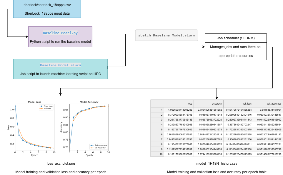
Figure: An illustration of the Baseline Model workflow.
Post-Analysis on Baseline_Model.py
After running Baseline_Model.slurm, use post_analysis_Baseline_Model.ipynb (recreated below) to run analysis on the results.
Step 0: Import modules
import os
import pandas as pd
import matplotlib.pyplot as plt
import numpy as np
%matplotlib inline

# Helper function:

def plot_training_history(history_file, subtitle):
    """
    Creates and displays a two-panel subplots to visualize the progress
    of a model training run.
    The left panel contains the training and validation loss vs. epochs;
    the right panel contains the training validation accuracy vs. epochs.
    This function expects to read the training history from a CSV file,
    which contains loss & accuracy values computed with training and validation
    sets.

    Args:
      history_file (str): The pathname of the CSV file.
      subtitle (str): A string to append to the plot's titles.
    """
    # Initialize the subplots
    fig, axs = plt.subplots(1, 2, figsize=(10,4))

    # The history file contains the data to plot
    epochMetrics = pd.read_csv(history_file)
    # The epoch values corresponds to the index of the read dataframe,
    # which will be 0, 1, 2, ...
    epochs = np.array(epochMetrics.index)

    # Plot the loss subplot
    axs[0].plot(epochs, epochMetrics['loss'])
    axs[0].plot(epochs+1, epochMetrics['val_loss'])

    # Code to add the title, axis labels, etc.
    axs[0].set_title("Model Loss: " + subtitle)
    axs[0].legend(["Train Loss", "Val Loss"])
    axs[0].set_ylabel("Loss")
    axs[0].set_xlabel("Epochs")
    axs[0].set_xlim(xmin=0)
    axs[0].set_ylim(ymin=0)

    # Plot the accuracy subplot
    axs[1].plot(epochs, epochMetrics['accuracy'])
    axs[1].plot(epochs+1, epochMetrics['val_accuracy'])

    # Code to add the title, axis labels, etc.
    axs[1].set_title("Model Accuracy: " + subtitle)
    axs[1].legend(["Train Accuracy", "Val Accuracy"])
    axs[1].set_ylabel("Accuracy")
    axs[1].set_xlabel("Epochs")
    axs[1].set_xlim(xmin=0)

    # create space between the plots
    plt.subplots_adjust(left=None, bottom=None, right=None, top=None, \
                        wspace=0.4, hspace=0.4)
    plt.show()
Step 1A: Discovery of all the results
## We know all of the output file names (because we set them)
## So for now, just use the set file paths

csvFile = './model_1H18N_history.csv'
imgPath = "./loss_acc_plot.png"
modelPath = "./model_1H18N.h5"
Step 1B: Load the results
# Load in the csv file containing the loss, accuracy, val_loss, and val_accuracy

df = pd.read_csv(csvFile)
print(df)
       loss  accuracy  val_loss  val_accuracy
0  1.063700  0.705481  0.491797      0.891515
1  0.372994  0.915958  0.298905      0.933023
2  0.261755  0.938790  0.233927      0.941592
3  0.213864  0.948938  0.197564      0.953841
4  0.183789  0.956024  0.172288      0.956313
5  0.161887  0.961403  0.152240      0.963307
6  0.144552  0.965257  0.136864      0.966402
7  0.130466  0.967262  0.124825      0.967921
8  0.118756  0.968905  0.113000      0.971620
9  0.108179  0.971418  0.103512      0.971437
# Utilize the helper function to plot the history
plot_training_history(csvFile,
                      subtitle="1H18N Baseline Model")
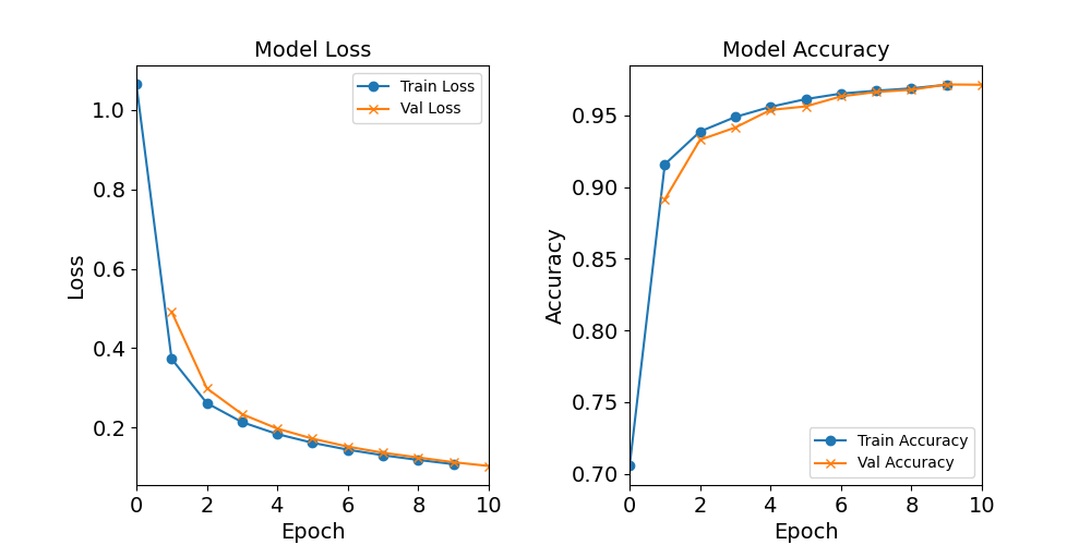
Figure: The model’s loss and accuracy as a function of epochs from the baseline model (1H18N)
## Load in the model, though for this case, we do not need this
#model_1H = keras.saving.load_model("./model_1H18N.h5")
Step 2: Validation of Model Training: Visual Inspection
As stated above, this step is easiest done by graphically inspecting the training history graphs.
1) Inspect if the trainings did not go as expected. In other words, check for any anomalies in the training trends. They should behave in the following manner:
-
Initially, the loss drops rapidly, but it continues to drop monotonously, and is slowing down as with increasing epochs.
-
The accuracy increases rapidly before leveling off slowly.
-
The accuracy did not show a drop when computed with validation dataset, showing that there is no overfitting here.
2) Visually (or numerically) check for convergence (e.g. check the loss or accuracy for the last 4-5 epochs; what their slopes look like in this region; any fluctuations?)
3) Observe the final accuracy. (We will do this more carefully in the next phase)
The training did behave as expected.
The training loss is decreasing as the number of epochs increases, while the accuracy increases.
There are no major anomalies (such as any random spikes or dips).
It looks like both the accuracy and loss functions are starting to converge.
Therefore, this model behaves as expected.
Step 3: Create a Result DataFrame
This result DataFrame should include the performance metrics from the last epoch for each of the experiments (of the same experiment type). The value of the varying hyperparameter should be in the first column.
# Fetch the loss, accuracy, val_loss, and val_accuracy from the last epoch
# (should be the last row in the CSV file unless there's something wrong
# during the traning)
lastEpochMetrics = df.iloc[-1, :].to_dict()
# Attach the "neurons" value
lastEpochMetrics["hidden_neurons"] = 18

df_HN = pd.DataFrame([lastEpochMetrics],
                     columns=["hidden_neurons", "loss", "accuracy", "val_loss", "val_accuracy"])
print(df_HN)
 hidden_neurons      loss  accuracy  val_loss  val_accuracy
0              18  0.106375  0.976138  0.101126      0.977003
Step 4: Saving the intermediate DataFrame
Save the intermediate DataFrame to be read in during the post-analysis phase.
df_HN.to_csv("post_processing_Baseline_Model.csv", index=False)
Step 5: Analysis phase: visualizing the results
The post-analysis phase is for comparing among experiments. Since this post-analysis script is for one model’s results, this step can be skipped.
Running Experiments Utilizing Command Line Arguments (NN_Model_1H)
We just created a Python and SLURM script that runs one model with fixed hyperparameters. However, we want to be able to utilize batch scripts to run multiple experiments at the same time.
One way to accomplish this is by utilizing command line arguments. Command line arguments will add the capability of defining hyperparameters in the SLURM file (or on the terminal). This will allow the user to create one (flexible) Python script with multiple SLURM scripts.
With this one to many convention, we must establish an organization method. We can utilize the naming convention established in the previous episode.
MODEL_DIR = model_1H + HIDDEN_NEURONS + N_lr + LEARNING_RATE + _bs + BATCH_SIZE + _e + EPOCHS
The python script will create an output directory and give it this MODEL_DIR name.
This output directory will contain loss_acc_plot.png, model_history.csv, model_metadata.json and model_weights.h5.
The JSON file will be explained shortly, but for now,
just assume it is another (unique) output for one experiment
(i.e. run of the Python script).
The MODEL_DIR name will also be used to name the SLURM output file, along with the job number.
So, each experiment/run will have it’s own corresponding output directory and SLURM output file named according to the hyperparameters used.
Implementing Command Line Arguments
Duplicate Baseline_Model.py and rename the new copy NN_Model_1H.py.
Make the following changes to the code.
0) (Optional) Change the heading of the file.
"""
NN_Model_1H.py

Python script for model tuning experiments.
Running this script requires four arguments on the command line:

    python3  NN_Model_1H.py  HIDDEN_NEURONS  LEARNING_RATE  BATCH_SIZE  EPOCHS

"""
1) Import the additional libraries.
# ## 1. Loading Python Libraries


import os
import sys

import pandas as pd
import numpy as np

# CUSTOMIZATIONS (optional)
np.set_printoptions(linewidth=1000)

# tools for deep learning:
import tensorflow as tf
import tensorflow.keras as keras

# Import ML toolbox functions
from sherlock_ML_toolbox import load_prep_data_18apps, split_data_18apps, \
NN_Model_1H, plot_loss, plot_acc, combine_loss_acc_plots, fn_dir_tuning_1H

import time
import json
2) Define the hyperparameters at the top and assign them
the command line argument values using sys.argv.
We create a standard model output directory name that
is based on the hyperparameter values.
As explained above, having a standard name assists in maintaining the
experiments and during post-analysis and post-processing.
Next, print the hyperparameters to the output file.
# Utilize command line arguments to set the hyperparameters
HIDDEN_NEURONS = int(sys.argv[1])
LEARNING_RATE = float(sys.argv[2])
BATCH_SIZE = int(sys.argv[3])
EPOCHS = int(sys.argv[4])

# Create model output directory
model_name = fn_dir_tuning_1H("",
                 HIDDEN_NEURONS, LEARNING_RATE,
                 BATCH_SIZE, EPOCHS)
MODEL_DIR = model_name
if not os.path.exists(MODEL_DIR):
    os.makedirs(MODEL_DIR)

# print hyperparameter information
print()
print("Hyperparameters for the training:")
print("  - hidden_neurons:", HIDDEN_NEURONS)
print("  - learning_rate: ", LEARNING_RATE)
print("  - batch_size:    ", BATCH_SIZE)
print("  - epochs:        ", EPOCHS)
print()
Keep step 2: Loading Sherlock Applications Data the same (including the print statements).
3) Then, change all (variable) references to the hardcoded hyperparameters.
model_1H = NN_Model_1H(HIDDEN_NEURONS, LEARNING_RATE)
model_1H_history = model_1H.fit(train_features,
                                train_L_onehot,
                                epochs=EPOCHS, batch_size=BATCH_SIZE,
                                validation_data=(val_features, val_L_onehot),
                                verbose=2)
4) Next, change the output file names using the model directory path created above. This will allow all of the output files to share a common name and be contained in their respective model directory.
history_file = os.path.join(MODEL_DIR, 'model_history.csv')
plot_file = os.path.join(MODEL_DIR, 'loss_acc_plot.png')
model_file = os.path.join(MODEL_DIR, 'model_weights.h5')
metadata_file = os.path.join(MODEL_DIR, 'model_metadata.json')
5) Then, add the additional step of creating the metadata. Using JSON allows the user to easily read and write the structured metadata. It saves name-value pairs that can be queried.
# Because of the terseness of Keras API, we create our own definition
# of a model metadata.

# timestamp of the results (at the time of saving)
model_1H_timestamp = time.strftime('%Y-%m-%dT%H:%M:%S%z')
# last epoch results is a key-value pair (i.e. a Series)
last_epoch_results = history_df.iloc[-1]

model_1H_metadata = {
    # Our own information
    'dataset': 'sherlock_18apps',
    'keras_version': tf.keras.__version__,
    'SLURM_JOB_ID': os.environ.get('SLURM_JOB_ID', None),
    'timestamp': model_1H_timestamp,
    'model_code': MODEL_DIR,
    'optimizer': 'Adam',
    # the number of hidden layers will be deduced from the length
    # of the hidden_neurons array:
    'hidden_neurons': [HIDDEN_NEURONS],
    'learning_rate': LEARNING_RATE,
    'batch_size': BATCH_SIZE,
    'epochs': EPOCHS,
    # Some results
    'last_results': {
        'loss': round(last_epoch_results['loss'], 8),
        'accuracy': round(last_epoch_results['accuracy'], 8),
        'val_loss': round(last_epoch_results['val_loss'], 8),
        'val_accuracy': round(last_epoch_results['val_accuracy'], 8),
    }
}

with open(metadata_file, 'w') as F:
    json.dump(model_1H_metadata, F, indent=2)
Metadata
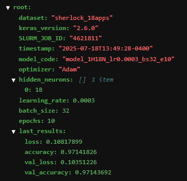
Recall from the previous episode, that metadata should be collected during each experiment. The metadata collected is decided by the user and should contain helpful information to the user. This should include information about the compute environment or information to help with troubleshooting, such as the
keras_versionandtimestamp. It should also contain information about the experiment, such as the hyperparameters. It can also contain “summary” information, such aslast_results, which saves the last epoch results.
Figure: The metadata saved in the JSON file for the baseline model. Note, there might be slight differences between your JSON data and this one. For example, the SLURM_JOB_ID, keras_version, and timestamp might vary. The last_results will vary as well, but should be similar.
Creating SLURM Script with Command Line Arguments
First, duplicate the Baseline_Model.slurm file and rename it to NN_Model_1H.slurm.
Then, change the name of the job:
#SBATCH -J model-tuning-1H
Then, add the block that will take in
the command line arguments.
Note, the actual values will be set in
a different slurm script, or can be passed within the sbatch command (on the terminal).
Make sure that the order of the variables in the Python and SLURM script match!
The values (syntax-wise) can be defined a couple different ways.
One way is by doing --[variableName] [value].
Another is by doing "".
# HYPERPARAMS_LIST contains four arguments,
# which must be given in the command-line argument:
#   * the number of hidden neurons
#   * the learning rate
#   * the batch size
#   * the number of epochs to train

HIDDEN_NEURONS=$1
LEARNING_RATE=$2
BATCH_SIZE=$3
EPOCHS=$4
Then, add the hyperparameters to the last line.
$CRUN $CRUN_ENVS_FLAGS python3 NN_Model_1H.py "$HIDDEN_NEURONS" "$LEARNING_RATE" "$BATCH_SIZE" "$EPOCHS"
Run NN_Model_1H.slurm by passing in the arguments into the command line.
In the terminal, run the
NN_Model_1H.slurm. In this example, the number of hidden neurons in the first layer is 18, the learning rate is 0.0003, the batch size is 32, and the number of epochs is 10.sbatch NN_Model_1H.slurm 18 0.0003 32 10Since these were the same hyperparameters used in
Baseline_Model.py, the results should look the same.
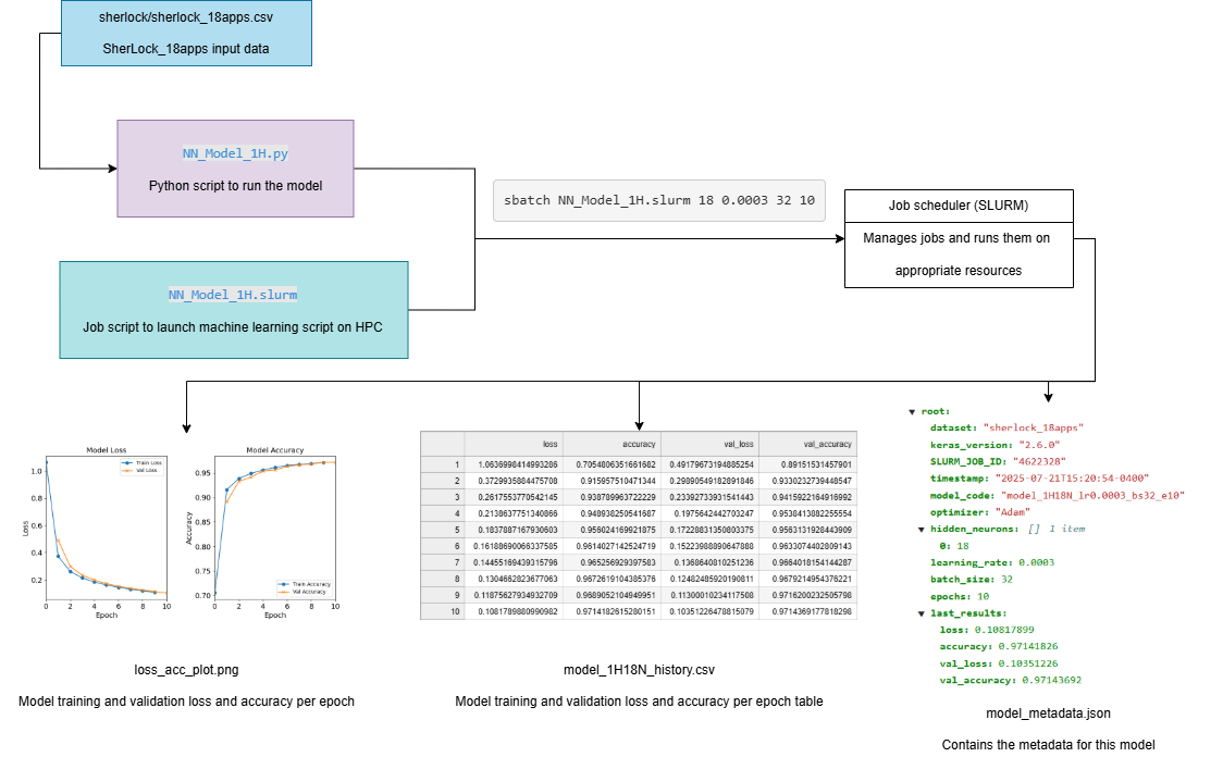
Figure: The workflow for running model tuning experiments utilizing command line arguments.
Using a Master Launcher Script to Launching a Series of Jobs for a Certain Hyperparameter Scanning Task
We can use a master launcher script with a “for loop,” to allow for the launching of a series of jobs for a certain hyperparameter scanning task. This can be used to replicate the experiments from before, within the previous episode, Tuning Neural Network Models for Better Accuracy.
Create another directory named scan-hidden-neurons and create a submit-scan-hidden-neurons.sh file that will submit multiple jobs that vary the number of hidden neurons
(in the first layer).
Make sure to also copy the NN_Model_1H.slurm, NN_Model_1H.py, sherlock_ML_toolbox.py, and the sherlock data/directory files.
Note, for the NN_Model_1H.py file, change the metadata section’s model code to
'model_code': "1H"+str(HIDDEN_NEURONS)+"N",
since this is the hyperparameter that is changing.
To do so, define the hyperparameters at the top of the script that do not vary.
Then, create a for loop with the varying hyperparameter with the values to experiment.
Next, define JOBNAME, which will be the name of the output file.
This will follow the same naming convention for the output directory names.
Then, use the sbatch command to call NN_Model_1H.slurm with the given variable values.
#!/bin/bash
#HIDDEN_NEURONS= -- varied
LEARNING_RATE=0.0003
BATCH_SIZE=32
EPOCHS=30

for HIDDEN_NEURONS in 1 2 4 8 12 18 40 80; do
    JOBNAME=model_1H${HIDDEN_NEURONS}N_lr${LEARNING_RATE}_bs${BATCH_SIZE}_e${EPOCHS}
    echo "Training for hyperparams:" "$HIDDEN_NEURONS"  "$LEARNING_RATE"  "$BATCH_SIZE"  "$EPOCHS"
    sbatch -J "$JOBNAME"  NN_Model_1H.slurm  "$HIDDEN_NEURONS"  "$LEARNING_RATE"  "$BATCH_SIZE"  "$EPOCHS"
done
For this script, 8 different jobs will be spawned, each with a
0.0003 learning rate, batch size of 32, and 30 epochs.
Each of the 8 jobs will have a different amount of hidden neurons (in the first layer).
So, the first job will call NN_Model_1H.slurm with a 0.0003 learning rate, batch size of 32, and 30 epochs, and with 1 hidden neuron.
The second job will call NN_Model_1H.slurm with a 0.0003 learning rate, batch size of 32, and 30 epochs, and with 2 hidden neurons.
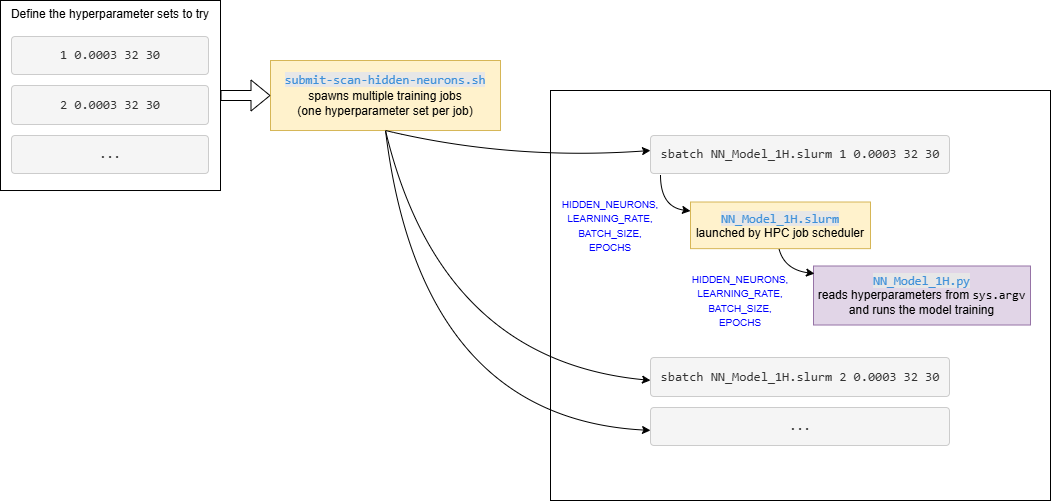
Figure: Diagram showing the workflow for the hyperparameter HPC scan.
Note that this is for the hidden neurons experiment type,
so the workflow will be slighty different for each experiment type.
For example, the submit-scan-hidden-neurons.sh will be
replaced with the relevant submit-scan- file.
Run the experiments. Make sure that all of the relevant files were copied into the current directory!
Additional Epochs
To get a better understanding of how the hyperparameters affect the accuracy of the model, additional epochs were added. The number of epochs increase from 10 to 30. Note that this change is implemented in the
submit-scan-hidden-neurons.shscript.
Additional Hidden Neurons
Perform the following additional experiments: Use the relevant files to create three different models/experiments with 256, 512, and 1024 hidden neurons.
Solution
There are two different ways to do this. You can use the command line:
sbatch NN_Model_1H.slurm 256 0.0003 32 30
sbatch NN_Model_1H.slurm 512 0.0003 32 30
sbatch NN_Model_1H.slurm 1024 0.0003 32 30
OR
Modify the for loop in
submit-scan-hidden-neurons.shto also run 256, 512, and 1024 hidden neurons.for HIDDEN_NEURONS in 256 512 1024; do
Post-Processing Results from submit-scan-hidden-neurons.sh (post_processing.ipynb)
After running submit-scan-hidden-neurons.sh, usepost_processing.ipynb (also reproduced below) to analyze the results.
Step 0: Import Modules and Define Helper Functions
import os
import sys

import pandas as pd
import matplotlib.pyplot as plt
import numpy as np

from sherlock_ML_toolbox import fn_out_history_1H, fn_out_history_XH

%matplotlib inline

def plot_training_history(history_file, subtitle):
    """
    Creates and displays a two-panel subplots to visualize the progress
    of a model training run.
    The left panel contains the training and validation loss vs. epochs;
    the right panel contains the training validation accuracy vs. epochs.
    This function expects to read the training history from a CSV file,
    which contains loss & accuracy values computed with training and validation
    sets.

    Args:
      history_file (str): The pathname of the CSV file.
      subtitle (str): A string to append to the plot's titles.
    """
    # Initialize the subplots
    fig, axs = plt.subplots(1, 2, figsize=(10,4))

    # The history file contains the data to plot
    epochMetrics = pd.read_csv(history_file)
    # The epoch values corresponds to the index of the read dataframe,
    # which will be 0, 1, 2, ...
    epochs = np.array(epochMetrics.index)

    # Plot the loss subplot
    axs[0].plot(epochs, epochMetrics['loss'])
    axs[0].plot(epochs+1, epochMetrics['val_loss'])

    # Code to add the title, axis labels, etc.
    axs[0].set_title("Model Loss: " + subtitle)
    axs[0].legend(["Train Loss", "Val Loss"])
    axs[0].set_ylabel("Loss")
    axs[0].set_xlabel("Epochs")
    axs[0].set_xlim(xmin=0)
    axs[0].set_ylim(ymin=0)

    # Plot the accuracy subplot
    axs[1].plot(epochs, epochMetrics['accuracy'])
    axs[1].plot(epochs+1, epochMetrics['val_accuracy'])

    # Code to add the title, axis labels, etc.
    axs[1].set_title("Model Accuracy: " + subtitle)
    axs[1].legend(["Train Accuracy", "Val Accuracy"])
    axs[1].set_ylabel("Accuracy")
    axs[1].set_xlabel("Epochs")
    axs[1].set_xlim(xmin=0)

    # create space between the plots
    plt.subplots_adjust(left=None, bottom=None, right=None, top=None, \
                        wspace=0.4, hspace=0.4)
    plt.show()
Step 1: Discover and Load the Results
# The number of neurons for each experiment/model
# (adjust the values to the actual experiments that you ran)
listHN = [1, 2, 4, 8, 12, 18, 40, 80, 256, 512, 1024]

# base folder of the experiment
dirPathHN = "scan-hidden-neurons"
Step 2: Validating of Model Training: Visual Inspection
for i, HN in enumerate(listHN):
    plot_training_history(fn_out_history_1H(dirPathHN, HN, 0.0003, 32, 30),
                          subtitle="1H"+str(HN)+"N")
Based on the plots shown above, inspect whether the training runs went as expected.
1) Visually inspect for any anomalies. Note the runs that produce “abnormal training trends”, i.e., where the “loss vs epochs” and/or “accuracy vs epochs” curves exhibit a different behavior from what shown in the earlier 2-panel plot.
2) Visually (or numerically) check for convergence (e.g. check the loss or accuracy for the last 4-5 epochs; what their slopes look like in this region; any fluctuations?)
3) Observe the differences in the final accuracies as a result of different hidden_neurons values. (We will do this more carefully in the next phase)
Perform these visual inspections.
Solution
Both the loss and accuracy graphs look abnormal for the
1H1N,1H2N, and1H4Nmodels. They exhibit a “local minimum shelf” (around epochs 5-15) before finding a better minimum. This suggests that these models are struggling to properly learn the patterns in the data, because the number of the hidden neurons are simply inadequate. In the lowerhidden_neurons, it is quite obvious that the accuracy is still climbing noticeably (in the plot), which means that training convergence hasn’t been achieved well. For example, take a close look at1H12Nrun.The 1H1N is a total failure (accuracy is well below 0.5); but neither 1H2N and 1H4N is good especially if we see at higher
hidden_neuronsthey exhibit accuracies well above 99%.Runs with higher
hidden_neuronsare better: They started at higher initial accuracies and climbed closer to 1.00 (visually speaking).
Step 3: Create a Result DataFrame for the hidden_neurons Hyperparameter Scan
We want to investigate the changes of the final metrics as the input hyperparameter
is varied (in this case, hidden_neurons).
This investigation will be done later, but for now, we will collect these final
metrics with the relevant hyperparameter(s) and metadata into an intermediate
DataFrame and save them as a CSV file.
# This is the epoch number from which we want to extract results
# for analysis of hyperparameter effects
# (corresponding to epoch #30)
lastEpochNum = 29
We use a loop to read all the output files from this experiment
and gather the final metrics into a new dataframe called df_HN
(where HN is, again, a shorthand for “hidden neurons tuning experiment”).
The sequence of the varied hyperparameter specified in listHN,
defined aboves.
This can be done via different methods, but we will focus on the via a temporary data structure method.
In this method, we will construct and fill a temporary data structure (all_lastEpochMetrics) dynamically before forming the dataframe.
This approach is useful when the size of the data (e.g. total number of rows) is not known a priori.
The following is a simplified loop which shows the logic of this intermediate data construction:
all_lastEpochMetrics = []
# Fill in the rows for the DataFrame
for HN in listHN:
    # Read the history CSV file and get the last row's data,
    # which corresponds to the last epoch data.
    #run_subdir = "model_1H" + str(HN) + "N_lr0.0003_bs32_e30"
    #result_csv = os.path.join(dirPathHN, run_subdir, "model_history.csv")
    result_csv = fn_out_history_1H(dirPathHN, HN, 0.0003, 32, 30)
    print("Reading:", result_csv)
    epochMetrics = pd.read_csv(result_csv)
    # Fetch the loss, accuracy, val_loss, and val_accuracy from the last epoch
    # (should be the last row in the CSV file unless there's something wrong
    # during the traning)
    lastEpochMetrics = epochMetrics.iloc[lastEpochNum, :].to_dict()
    # Attach the "neurons" value
    lastEpochMetrics["hidden_neurons"] = HN
    all_lastEpochMetrics.append(lastEpochMetrics)
Reading: scan-hidden-neurons/model_1H1N_lr0.0003_bs32_e30/model_history.csv
Reading: scan-hidden-neurons/model_1H2N_lr0.0003_bs32_e30/model_history.csv
Reading: scan-hidden-neurons/model_1H4N_lr0.0003_bs32_e30/model_history.csv
Reading: scan-hidden-neurons/model_1H8N_lr0.0003_bs32_e30/model_history.csv
Reading: scan-hidden-neurons/model_1H12N_lr0.0003_bs32_e30/model_history.csv
Reading: scan-hidden-neurons/model_1H18N_lr0.0003_bs32_e30/model_history.csv
Reading: scan-hidden-neurons/model_1H40N_lr0.0003_bs32_e30/model_history.csv
Reading: scan-hidden-neurons/model_1H80N_lr0.0003_bs32_e30/model_history.csv
Reading: scan-hidden-neurons/model_1H256N_lr0.0003_bs32_e30/model_history.csv
Reading: scan-hidden-neurons/model_1H512N_lr0.0003_bs32_e30/model_history.csv
Reading: scan-hidden-neurons/model_1H1024N_lr0.0003_bs32_e30/model_history.csv
df_HN = pd.DataFrame(all_lastEpochMetrics,
                     columns=["hidden_neurons", "loss", "accuracy", "val_loss", "val_accuracy"])

print(df_HN)
    hidden_neurons      loss  accuracy  val_loss  val_accuracy
0                1  1.945121  0.319691  1.947505      0.320510
1                2  1.051278  0.682108  1.061323      0.682804
2                4  0.463814  0.907489  0.460035      0.910356
3                8  0.183243  0.952651  0.183629      0.950912
4               12  0.070112  0.985663  0.068991      0.985389
5               18  0.045203  0.990570  0.043723      0.990589
6               40  0.016035  0.996434  0.017410      0.996375
7               80  0.007796  0.998654  0.011362      0.998425
8              256  0.003840  0.999515  0.007077      0.999194
9              512  0.002919  0.999606  0.009277      0.999249
10            1024  0.003308  0.999593  0.006825      0.999231
Step 4: Save the Intermediate DataFrame
df_HN.to_csv("post_processing_hpc_neurons.csv", index=False)
Learning Rate and Batch Size Experiments
Learning Rate Experiment
To recreate the experiment: test with different learning rates of 0.0003, 0.001, 0.01, and 0.1. First, create the folder scan-learning-rate.
Make sure that this directory includes the sherlock data/directory, NN_Model_1H.slurm,
NN_Model_1H.py, and sherlock_ML_toolbox.py.
Next, create submit-scan-learning-rate.sh.
This script will be similar to the submit-scan-hidden-neurons.sh.
#!/bin/bash

HIDDEN_NEURONS=18
#LEARNING_RATE= -- varied
BATCH_SIZE=32
EPOCHS=30

for LEARNING_RATE in 0.0003 0.001 0.01 0.1; do
    #JOBNAME=model-tuning-1H${HIDDEN_NEURONS}N
    #OUTDIR=model_1H${HIDDEN_NEURONS}N_lr${LEARNING_RATE}_bs${BATCH_SIZE}_e${EPOCHS}
    JOBNAME=model_1H${HIDDEN_NEURONS}N_lr${LEARNING_RATE}_bs${BATCH_SIZE}_e${EPOCHS}
    echo "Training for hyperparams:" "$HIDDEN_NEURONS"  "$LEARNING_RATE"  "$BATCH_SIZE"  "$EPOCHS"
    sbatch -J "$JOBNAME"  NN_Model_1H.slurm  "$HIDDEN_NEURONS"  "$LEARNING_RATE"  "$BATCH_SIZE"  "$EPOCHS"
done
Change the Python script’s model_1H_metadata model code line to the following.
'model_code': "lr" + str(LEARNING_RATE),
   learning_rate      loss  accuracy  val_loss  val_accuracy
0         0.0003  0.045203  0.990570  0.043723      0.990589
1         0.0010  0.018579  0.995926  0.021447      0.995862
2         0.0100  0.021298  0.995395  0.024532      0.995386
3         0.1000  0.444514  0.921821  0.340468      0.921012
Perform the Post-Processing for the Learning Rate Experiments
Solution
A very small learning rate results in slower, but smoother progression in
val_accuracy. After 30 iterations, it still hovers at 0.9905 and the rate of change is still about 0.0005.A larger learning rate (0.01) results in faster convergence, but the result (as represented by
val_accuracy) has more noise. The average accuracy is 0.995, but the noise is on the order of 0.001-0.002, which is quite large. The loss and accuracy plots start looking abnormal at this learning rate, but it still does follow the general expected shape of the metrics-vs-epoch curves.An even larger learning rate (0.1) results in totally erratic training. It is truly unusable. This tells us that learning rate 0.1 should not be used because it messes up the learning process.
Batch Size Experiment
The batch size experiment will be conducted similarly to the learning rate experiment.
To recreate the experiment: test with different batch sizes: 16, 32, 64, 128, 512, 1024,
create the output directory scan-batch-size.
Make sure that this directory includes ther sherlock data/directory, NN_Model_1H.slurm,
NN_Model_1H.py, and sherlock_ML_toolbox.py.
Next, create submit-scan-batch-size.sh.
This script will be similar to the submit-scan-hidden-neurons.sh.
#!/bin/bash

HIDDEN_NEURONS=18
LEARNING_RATE=0.0003
#BATCH_SIZE= --varied
EPOCHS=30

for BATCH_SIZE in 16 32 64 128 512 1024; do
    #JOBNAME=model-tuning-1H${HIDDEN_NEURONS}N
    #OUTDIR=model_1H${HIDDEN_NEURONS}N_lr${LEARNING_RATE}_bs${BATCH_SIZE}_e${EPOCHS}
    JOBNAME=model_1H${HIDDEN_NEURONS}N_lr${LEARNING_RATE}_bs${BATCH_SIZE}_e${EPOCHS}
    echo "Training for hyperparams:" "$HIDDEN_NEURONS"  "$LEARNING_RATE"  "$BATCH_SIZE"  "$EPOCHS"
    sbatch -J "$JOBNAME"  NN_Model_1H.slurm  "$HIDDEN_NEURONS"  "$LEARNING_RATE"  "$BATCH_SIZE"  "$EPOCHS"
done
Also, change the model code in the model_1H_metadata section to be the following.
'model_code': "bs"+str(BATCH_SIZE),
   batch_size      loss  accuracy  val_loss  val_accuracy
0          16  0.023600  0.994557  0.023432      0.994763
1          32  0.045203  0.990570  0.043723      0.990589
2          64  0.062618  0.985123  0.064284      0.984968
3         128  0.071049  0.985741  0.070776      0.985224
4         512  0.164543  0.959549  0.161178      0.959133
5        1024  0.276155  0.930404  0.273338      0.931119
Perform the Post-Processing for the Batch Size Experiments
Solution
All loss and accuracy graphs look “normal”. But a large batch size gives accuracy trend that are not quite typical, with a pronounced kink. A very small batch size gives higher accuracy
What is not shown here is the computation time. Looking at the raw training log shows that small batch size value leads to longer training (e.g. 12-13 secs per epoch for
batch_size=16 and 1 secs per epoch forbatch_size=1024). That is a big difference.Accuracy is worse at large batch sizes. Convergence is worse at large batch sizes. This means that large batch sizes are not advantageous. But, one might need to see what happens if the number of epochs are increased => will it help?
So, batch size does not really affect the stability of the training, but it affects the accuracy vs speed trade-off.
Multiple Layer Experiment
The multiple layer experiment requires more changes
to the Python script.
Make a copy of the previous NN_Model_1H.py and rename it to NN_Model_XH.py.
This new script will be flexible enough to accept a list of hidden neurons
with a comma separating the number of neurons in each layer.
So, for example, the user can input 18,18,18 which will create a model
with three layers, each containing 18 hidden neurons.
The model code (i.e. naming convention) stays the same, except that the
number before the H represents the number of layers,
which is followed by the number of neurons in each layer separated by N.
So, in the prior example, the model code would be model_3H18N18N18N_lr0.0003_bs32_e30.
As in the prior experiments, make sure to copy sherlock_ML_toolbox.py and the sherlock data.
Copy NN_Model_1H.slurm, which will be changed to NN_Model_XH.slurm.
Also, copy NN_Model_1H.py, which will be changed to NN_Model_XH.py.
Also, copy submit-scan-hidden-neurons.sh, which will change to submit-scan-layers.sh.
The Python code will change in the following ways.
- Add some import statements and change the
HIDDEN_NEURONSvariable to accept string.
# Import key Keras objects
from tensorflow.keras.models import Sequential
from tensorflow.keras.layers import Dense
from tensorflow.keras.optimizers import Adam

# Utilize command line arguments to set the hyperparameters
HIDDEN_NEURONS = str(sys.argv[1])
- After the reading in of the command line arguments,
create two variables,
MULT_LAYERSandNumLayers. The first is a boolean of if there are multiple layers, and the second represents the number of layers.
### Add the multi-layer additional code here
MULT_LAYERS = False
NumLayers = 1

# Create model output directory
# If it has a "," in it, it will have multiple layers
if "," in HIDDEN_NEURONS:
    MULT_LAYERS = True

    # Remove brackets and split by comma and space
    HIDDEN_NEURONS_INTS = HIDDEN_NEURONS.strip("[]")
    HIDDEN_NEURONS_INTS = HIDDEN_NEURONS_INTS.split(",")
    # Convert each element to an integer
    HIDDEN_NEURONS_INTS = list(map(int, HIDDEN_NEURONS_INTS))

    NumLayers = len(HIDDEN_NEURONS_INTS)

else:
    HIDDEN_NEURONS_INTS = [HIDDEN_NEURONS]

# Create model output directory
MODEL_DIR = fn_dir_tuning_XH("",
                 HIDDEN_NEURONS_INTS, LEARNING_RATE,
                 BATCH_SIZE, EPOCHS)
- Then, change the
NN_Model_1Hfunction toNN_Model_XH. If there are multiple layers, iterate through the list and create aDenselayer with that number of hidden neurons. Note, the first layer needs to be given a specific input shape.
def NN_Model_XH(hidden_neurons, learning_rate):
    """Definition of deep learning model with one or more dense hidden layer(s)"""
    # Use TensorFlow random normal initializer
    random_normal_init = tf.random_normal_initializer(mean=0.0, stddev=0.05)
    model = Sequential()
    if MULT_LAYERS:
        print("Number of layers: " + str(NumLayers))
        # The first layer should have a given input shape
        model.add(Dense(int(HIDDEN_NEURONS_INTS[0]), activation='relu', input_shape=(19,),
              kernel_initializer=random_normal_init)) # Hidden Layer
        for i in range(NumLayers-1):
            model.add(Dense(int(HIDDEN_NEURONS_INTS[i+1]), activation='relu',
              kernel_initializer=random_normal_init)) # Hidden Layer
    else:
        model.add(Dense(int(HIDDEN_NEURONS_INTS[0]), activation='relu', input_shape=(19,),
              kernel_initializer=random_normal_init)) # Hidden Layer
    model.add(Dense(18, activation='softmax',
              kernel_initializer=random_normal_init))  # Output Layer

    adam_opt = Adam(learning_rate=learning_rate, beta_1=0.9, beta_2=0.999, amsgrad=False)
    model.compile(optimizer=adam_opt,
                  loss='categorical_crossentropy',
                  metrics=['accuracy'])
    return model
- Since this uses a XH model, make sure to update the variable names.
model_XH = NN_Model_XH(HIDDEN_NEURONS_INTS, LEARNING_RATE)
model_XH_history = model_XH.fit(train_features,
                                train_L_onehot,
                                epochs=EPOCHS, batch_size=BATCH_SIZE,
                                validation_data=(val_features, val_L_onehot),
                                verbose=2)
history_df = pd.DataFrame(model_XH_history.history)
history_df.to_csv(history_file, index=False)

combine_loss_acc_plots(model_XH_history,
              plot_loss, plot_acc,
              loss_epoch_shifts=(0, 1),
              show=False,
              acc_epoch_shifts=(0, 1),
              save_path=plot_file)

model_XH.save(model_file)

# Because of the terseness of Keras API, we create our own definition
# of a model metadata.

# timestamp of the results (at the time of saving)
model_XH_timestamp = time.strftime('%Y-%m-%dT%H:%M:%S%z')
- Then, change the model_XH_metadata.
'timestamp': model_XH_timestamp,
'model_code': str(NumLayers)+"H"+str(HIDDEN_NEURONS)+"N",
- However, that is not how to actually set the metadata for the hidden neurons, so this code will fix it.
# Make sure the hidden neurons metadata is saved correctly!
# Make sure it is a list of integers
if MULT_LAYERS:
    model_XH_metadata['hidden_neurons'] = HIDDEN_NEURONS_INTS
    model_XH_metadata['model_code'] = model_XH_metadata['model_code'].replace(",", "N")
else:
    model_XH_metadata['hidden_neurons'] = [int(HIDDEN_NEURONS)]

with open(metadata_file, 'w') as F:
    json.dump(model_XH_metadata, F, indent=2)
Next, make sure to change NN_Model_1H.slurm to NN_Model_XH.slurm and
fix the Python file pointer and job name.
#SBATCH -J model-tuning-XH
$CRUN $CRUN_ENVS_FLAGS python3 NN_Model_XH.py "$HIDDEN_NEURONS" "$LEARNING_RATE" "$BATCH_SIZE" "$EPOCHS"
Finally, submit-scan-layers.sh.
First, change the for loop to test a model with a single layer with 18 hidden neurons, a model with two layers, each with 18 hidden neurons, a model with three layers, each with 18 hidden neurons, and finally a model with four layers, each with 18 hidden neurons.
for HIDDEN_NEURONS in "18" "18,18" "18,18,18" "18,18,18,18"; do
Second, use the following Linux commands to get the number of layers (used to input the correct JOBNAME). It will get the number of layers by changing the commas into new lines and then counting the number of new line characters. This is indented and is right after the for loop
    # get the number of layers: changes the commas into new lines, then counts that number of new lines
    H=$(echo $HIDDEN_NEURONS | sed -e 's/,/\n/g' | wc -l)
Then, set the JOBNAME correctly.
# So for example, "18,18,18,18" will produce an output file called model_4H18N18N18N18N_lr0.0003_bs32_e30
JOBNAME=model_${H}H${HIDDEN_NEURONS}N_lr${LEARNING_RATE}_bs${BATCH_SIZE}_e${EPOCHS}
    echo "Training for hyperparams:" "$HIDDEN_NEURONS"  "$LEARNING_RATE"  "$BATCH_SIZE"  "$EPOCHS"

# remove the , and then add the N after it for the Hidden Neurons
JOBNAME=$(printf '%s' "$JOBNAME" | sed 's/,/N/g')
Finally, update the file pointer to be NN_Model_XH.slurm.
sbatch -J "$JOBNAME" NN_Model_XH.slurm "$HIDDEN_NEURONS" "$LEARNING_RATE" "$BATCH_SIZE" "$EPOCHS"
Note: Make sure to re-run the post-processing notebook after completing all of the experiments!
Perform the Post-Processing for the Multiple Hidden Layers Experiments
Solution
No problems observed with stability / anomaly of the training runs.
Accuracy increased markedly when moving from 1 to 2 hidden layers, but not appear to improve after that.
Summary
We learned how to utilize the batch scheduler to more efficiently train and tune models.
First, we learned how to convert a Jupyter Notebooks with a neural network model into a Python script.
Refer to the Baseline_Model files.
Then, by utilizing the newly created Python script and
SLURM scripts.
Refer to the Baseline Model workflow.
Then, we introduced command-line arguments, allowing for the hyperparameters to be
defined in the SLURM scripts (instead of the Python scripts).
See the NN_Model_1H workflow.
Then, we recreated the experiments in Tuning Neural Network Models for Better Accuracy.
We streamlined this process by introducing a master launcher script to spawn multiple jobs for a certain
hyperparameter scanning task, allowing for the HPC to run the jobs in parallel.
The outputs from the experiments are compiled (and saved) as well as studied during the post-processing phase. The next phase is the post-analysis phase. During this phase, the user will load in the data from the post-processing phase and plot the relationship between one hyperparameter and the accuracy (from the last epoch) of the model.
Key Points
How scripting works by converting the notebook to job scripts
Build a simple toolset/skillset to create, launch, and manage the multiple batch jobs.
Use this toolset to obtain the big picture result after analyzing the entire calculation results as a set.
Use Jupyter notebook as the workflow driver instead of using it to do the heavy-lifting computations on it.