Deep Learning in the Real World
Overview
Teaching: 0 min
Exercises: 0 minQuestions
What kinds of layer can be built into a neural network?
Based on a particular scenario, what kind of layers should we use?
Objectives
Learning more advanced layer design
Neural Networks in Realistic Applications
Today, deep learning has been applied in many sophisticated applications which were previously thought impossible to do using computers. These include
- Face recognition, such as that used in smartphone face unlock;
- Object recognition, such as that used in computer vision system and self-driving cars;
- Text recognition, used in document scanning technologies;
- Voice recognition (e.g. Google Home, Alexa, smartphone voice input, and similar voice command systems);
- Conversational systems (think of: chat bots, ChatGPT);
- Medical diagnosis, such as tumor and other abnormality detection from medical imaging (MRI, CAT scan, X-ray…).
- Predictive analytics
- Supply chain optimization
- Recommendation system
In cybersecurity, neural network models have been deployed to filter spam emails, network intrusion and threat detection, detection of malware on a computer system, among other uses. Some real-world examples are listed in the following articles: “Five Amazing Applications of Deep Learning in Cybersecurity”; as well as “Google uses machine learning to catch spam missed by Gmail filters”.
These sophisticated applications call for more complex network architectures, which include additional types of layers, to help these networks in identifying patterns from spatial data points (collected from 2-D or 3-D images) and learning from sequences of data points (event correlation analysis, voice and video analysis). In this episode, we will briefly introduce various layers (beyond traditional dense neuron layers) that are used in state-of-the-art neural network models. We will also present an overview of several network architectures and their applications.
Types of Layers in Neural Networks
In order to build a neural network, one needs to know the different kinds layers which make up the building block of a neural network. In addition to the fully connected neuron layer (described in the previous episode), which constitutes the “thinking” part of the network, there are other types of layers that can provide spatial or temporal perception, “memory”, etc.
-
Dense layer (fully connected layer) is the classic neural network, in which every neuron connects to every point in the previous layer, and also connects to every point in the next layer. The previous or subsequent layer could be a neuron layer, or another kind of layer.

Figure 1: An example of a NN with three Dense layers (credit: Victor Gallego).
-
Convolution layer: A layer designed to capture local correlations/patterns in data that has spatial, temporal, or sequential order. This layer is frequently used in image-related tasks, but can be applied to speech recognition, voice detection, etc. A convolution layer applies a filter, or kernel (a set of weights), to the input to create a feature map. This filter applies a cross-correlation computation. Here is an illustration of convolution from a tutorial by Stanford University. Here are some real-life examples of applications of CNNs.
- Batch Normalization: Performs a transformation - a normalization - on the input, to bring the mean close to zero and the standard deviation close to one. This applies the theory that when learning about patterns in the data, relative differences among data points are more important than the absolute values. Normalization (in general) is important to make the training algorithm behave well (i.e., avoiding numerical instability). This layer applies the normalization differently during training and inference. During training, it uses the mean and standard deviation of the current batch (of inputs). During inference, it normalizes based on the moving average of the mean and standard deviation of the trained batches. The equations can be found here.
-
Pooling: This type of layer aggregates results over a specified size. It is frequently used in problems with spatial data (e.g., image related tasks). It reduces the dimensionality (or size/resolution) of the input by applying a sliding window transformation to the input. One popular pooling layer is the max-pooling layer, that applies a maximum operation to the data within the window. In this example (shown in the figure below), we will apply a max-pooling with a pooling window of 2x2. The pooling window is represented by the shaded portion. This 2x2 window will “slide” around the input applying a maximum operation, transforming the 3x3 input into a 2x2 output.
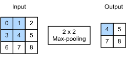
Figure 2: Applying a max-pooling (credit: Dive into Deep Learning).
-
Dropout: Temporarily randomly removing neurons/nodes and their corresponding connection. The goal is to reduce unnecessary feature dependencies and avoid overfitting in a neural network. This random removal is only done during the training phase; during inference, all neurons and connections will be turned on as usual. The exception being that the weights that were not affected by training (i.e. were removed), are scaled down. After each iteration/epoch, the set of neurons that are randomly selected change.
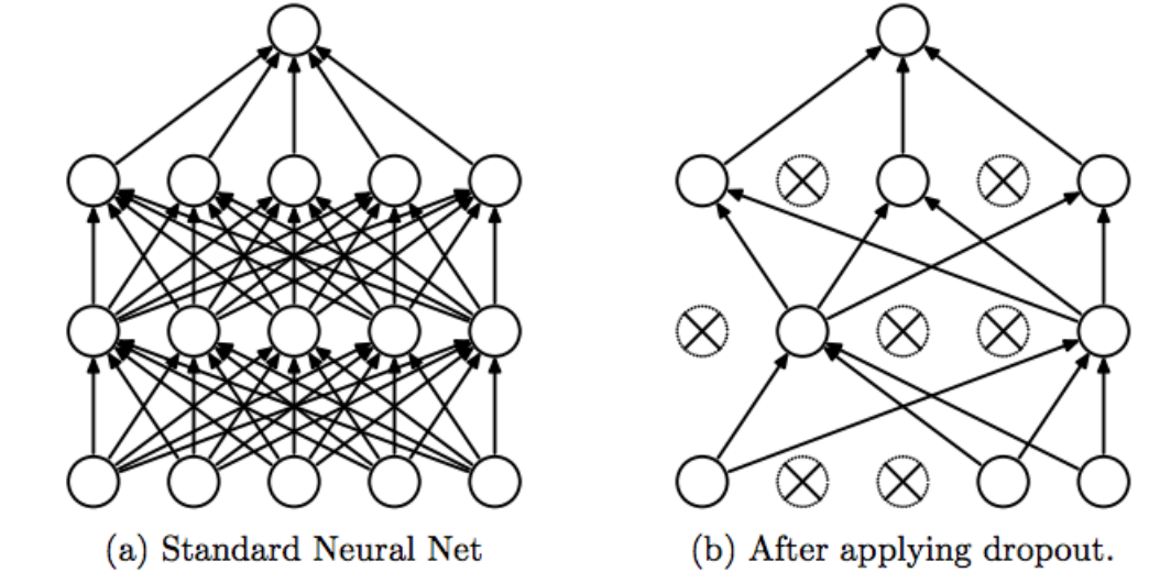 Figure 3: Dropout architecture (credit: Y. Bengio).
Activation Functions
There are several types of activation functions that can be used in modeling the neurons.
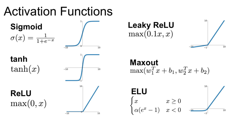
Figure 4: Some popular activation functions (credit: Medium user @krishnakalyan3).
The choice of activation functions is a hyperparameter that greatly affects the outcome of a neural network, and is problem and network architecture dependent. However, certain activation functions are more commonly used within certain neural networks. For example, CNNs typically use reLU. RNNs typically use tanh and sigmoid.
The Sigmoid function is the classic choice in the older days of neural networks. Recently, the ReLU (rectified linear unit) function has gained popularity because it is much cheaper to compute. The ELU (exponential linear unit) function is gaining popularity as it has been shown to perform faster and more accurately on some benchmark data.
Building a Neural Network
Building an appropriate network for a given task requires intuition and many experimentations to pick the best network. There are many tutorials and courses on deep learning which covers this topic (see the References section). A brief article by Jason Brownlee covers some of the approach, with some pointers for further reading. In reality, it will take a lot of trial-and-error to build a network that performs best for a certain task.
Other Neural Network Architectures
There are some more advanced layers which we will mention because it will be used in some exercises:
-
Multi-layer Perceptron (MLP): is a fully connected supervised neural network. It consists of an input layer, one or more (non-linear) hidden layers, and an output layer. This is the type of network that we created within this module.
-
Residual neural network (ResNet): utilizes residual learning. It uses skip connections, or “shortcut connections,” to group layers together that are “skipped”. These layers fit a residual mapping. It is used to avoid the problem of gradient vanishing among deep networks. It is used as the backbone for computer vision tasks.
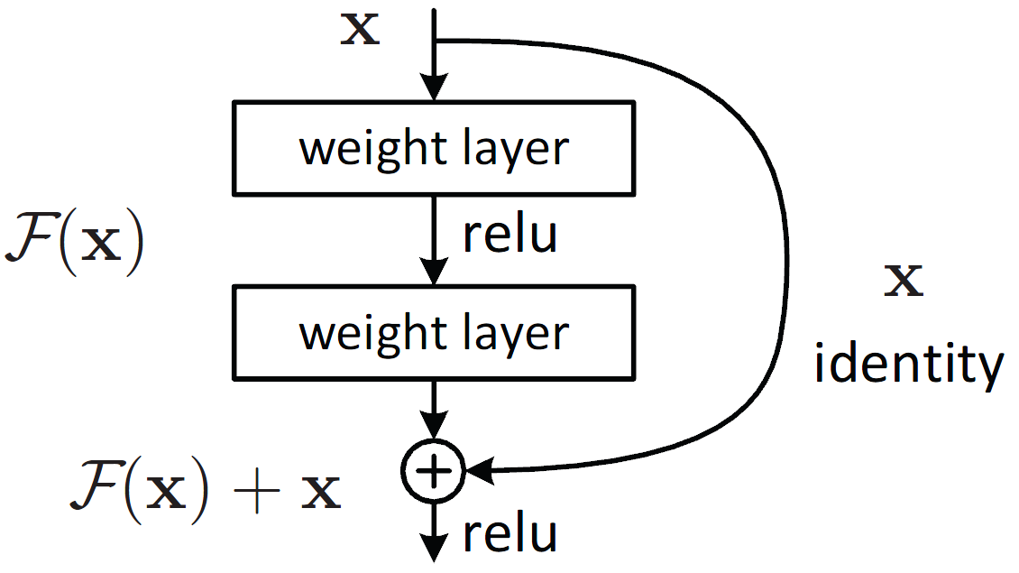
Figure 5: A residual block where x is the input, F(x) is the output vector and F(x) + x is the residual mapping to be learned (cite: He et. al.).
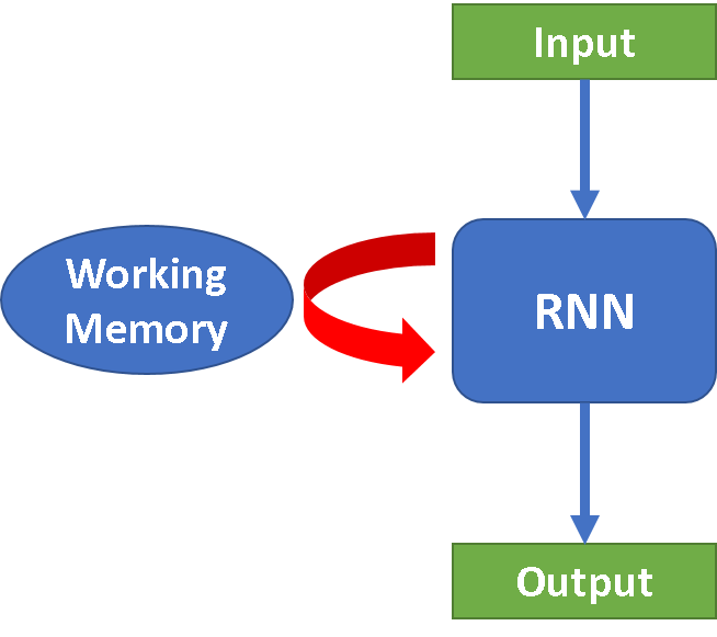
- Recurrent Neural Networks (RNN): this type of model assumes that the data provided is in a sequential order - usually text, speech, or time series data. The idea is that previous inputs (that are sequentially nearby) can influence the current output. This additional contextual information is stored as a “hidden state” and is also referred to as “memory” or “working memory.” Neurons are fed the current input and the hidden state from the previous step. RNN is good for processing sequence data for predictions but suffers from short-term memory.
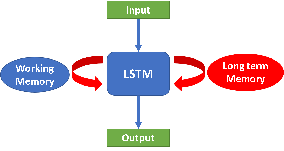
- Long Short-Term Memory (LSTM): It is a modified version of recurrent neural networks that assume longer-term contextual information affects future values. It introduces gates and an explicitly defined memory cell, which solves the gradient vanishing problem and makes it easier to remember past data in memory. In a nutshell, this layer provides some “remembering and forgetting” capability to a neural network to safeguard past information. LSTM is well-suited to classify, process, and predict sequential data given time lags of unknown duration. It is used for time-dependent problems such as speech recognition, natural language processing, etc.
-
Transformer Neural Network (TNN): It is another type of Neural Network. This NN is able to learn dependencies between sequences/elements that are further apart. It relies on attention - the mapping of queries, keys, and values to an output. The multi-head attention mechanism allows for parallel processing of sections of the data. The sections are assigned weights (i.e., importance). The weights for these sections make it “context-aware.”
Positional information is encoded within the Input Embedding and Positional Encoding layers. The Encoder consists of identical encoder layers that parallelly learns information within the input sequence. The shifted input sequence - the output sequence - is encoded with positional information within the Output Embedding and Positional Encoding layers. The Decoder consists of identical decoder layers. This combines the information from the encoder and the positional information from the previous decoder. The output is then transformed into a probability distribution. The inference step (most commonly a greedy search) is required to transform the output into a sequence. TNNs are well suited for language related tasks, such as translation.
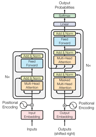
Figure 8: Transformer Neural Network architecture (cite: “Attention Is All You Need” (et. al.)).
“Transformers Explained Visually …” uses a text sequence example to illustrate how a TNN works.
-
Deep Belief Networks (DBNs): is a type of probabilistic deep learning algorithm that utilizes latent variables (or “hidden units”) and works on both supervised and unsupervised problems. DBN can be thought of as a stack of overlapping Restricted Boltzmann Machine (RBM) networks. Each RBM acting as a feature detector.
A RBM consists of a visible (input) layer and a hidden layer (that learns features). The hidden layer of one RBM model is the visible layer of the next RBM. A RBM is an energy-based model, where the energy (or “generative weights” or “latent variable”) value represents the probability of association between the hidden and visible units.
Training consists of an unsupervised pre-training phase and a supervised fine-tuning phase. Pre-training utilizes a greedy learning algorithm that employs a layer-by-layer approach to learn the generative weights. The goal of pre-training is to produce trained weights that directly represent the input data. Typically, a Contrastive Divergence algorithm is performed, consisting of a positive and negative phase. The positive phase samples the activation (function) of the visible layer to calculate probabilities for the activation of the hidden units. The negative phase does the opposite. Weights are updated after each pass. The fine-tuning phase utilizes the labeled data and a supervised learning algorithm (e.g. backpropogation).
These can be applied to image classification, text classification, etc. [Boesch] and [Kalita] himanshuit
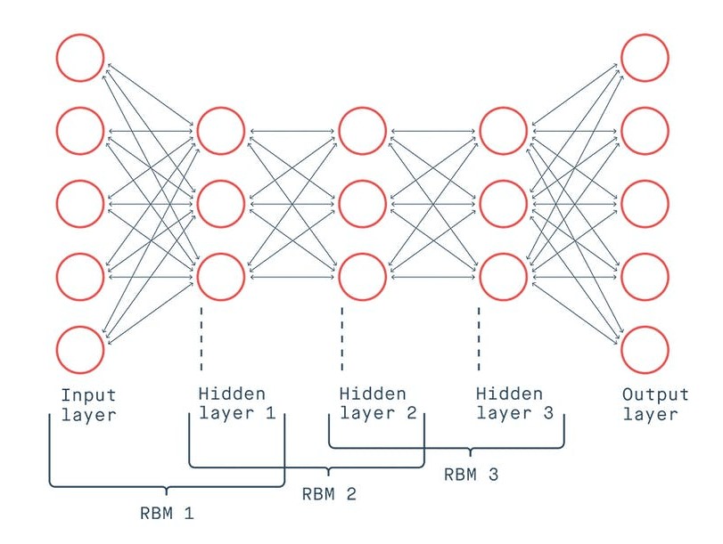
Figure 9: Deep Belief Network architecture (cite: “An Overview of Deep Belief Network (DBN) in Deep Learning” (Kalita)).
- Graph Neural Networks (GNNs): are designed to process and learn from data presented in a graphical manner. By modeling the relationships and connections between entities, GNNs make it possible to analyze and understand extremely complex systems. There are many varieties of data structures and scenarios that can be represented as a graph. Some of these include molecules, information networks, and genes. Some real-world applications include drug discovery: predicting molecular properties more efficiently; social recommendations; (credit: NVIDIA). GNNs unlock the potential of relational data and are paving the way for intelligent solutions in a wide range of industries.
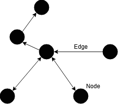
Figure 10: An illustration of a Graph Neural Network.
- Ensemble Models: combine the predictions of multiple individual models into a singular “ensemble meta-model.” This “meta-model” leverages the strengths of different models. Ensemble models focus less on the model tuning of individual models and more on how to combine the model results into a singular output. The types of models used can span different types of machine learning algorithms. An ensemble model usually combines algorithms that all excel in a type of task. For example, utilizing several time series predictive models together to make a more accurate prediction. “A comprehensive review on ensemble deep learning: Opportunities and challenges” provides an overview of ensemble models. It also provides several examples of ensemble model applications such as natural language processing (NLP), medical imaging, credit card fraud detection, etc.
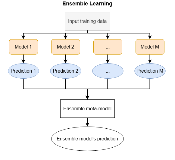
Figure 11: An illustration of an ensemble model.
Further Reading
There is an interesting chart by Fjodor Van Veen for well-known neural network types.
Key Points
Layer design