Problem Decomposition

Overview

Teaching: 0 min
Exercises: 0 min

Questions

How do we break a bigger computation into smaller pieces?

Objectives

Goal: break a big computation into smaller pieces that can be executed in parallel.

Problem Decomposition: Introduction

“Breaking up” an expensive computation into smaller parts that can be executed in parallel is referred to as problem decomposition or domain decomposition. Problem decomposition is very problem dependent. The method of problem decomposition may affect parallel efficiency. The best efficiency happens when the computation time per partition is (roughly) constant.

Problem Decomposition in One Dimension

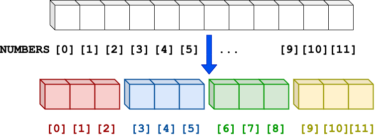
A very common scenario in problem-decomposition is the distribution of 𝑁 independent tasks as evenly as possible among 𝑃 workers. These N tasks can be thought of as items, tasks, array elements, grid points, etc. (This is to say that there is no interdependence among these tasks that would yield invalid results when executed in parallel.)

Problem Decomposition

Figure: Distribution of `N=12` numbers into `P=4` partitions, where each partition corresponds to a worker.

This approach works well to minimize the processing time if each task takes the same amount of time to process.

Dividing Items as Evenly as Possible in 1D

Create a subprogram to divide up the 𝑁 items as evenly as possible among the workers? Per MPI convention, we will label the workers with 𝑟=0,1,...(𝑃−1). There are different cases to consider when building an automatic 1-D domain decomposition.

Case 1: N perfectly divisible by P (define lower and upper bounds [L & U] for each worker’s rank. Example 1.1: N = 12; P = 4 Example 1.2: N = 100; P = 4

Case 2: Generalizing to N > P, but N/P has a remainder. Example 2.1: N = 14; P = 4 Example 2.2: N = 100; P = 7

Case 3: Generalization to N < P. Example 3.1: N = 5; P = 7

Consider, how many items does each worker receive (call this worksize)? Express it also in terms of N and P (i.e. as a mathematical formula involving 𝑁 and 𝑃). What are the inclusive lower (L) and exclusive upper (U) bounds of the original array received by worker with rank r? We follow the convention of Python for upper bound: where the elements assigned to a worker r will be NUMBERS[L], NUMBERS[L+1], … NUMBERS[U-1]. Note that by definition, worksize = U - L. Based on the manually worked-out L’s and U’s above, create the appropriate formulas for them involving N, P, and r.

Hints: you can use the integer division operator // or the int() function to yield integers instead of real numbers. The L and U variables should be an array with r as its index, as each worker is supposed to have a non-overlapping range of tasks (or data elements) to process.

Now, create a python solution to compute decomposition of N work items. Note, there are slightly different solutions. The sum of all worksize’s must equal to 𝑁, and there must not be any overlap or gap among the [𝐿,(𝑈−1)] intervals.

Use /handson/decomposition/solutions/range_decomp.ipynb.

def range_decomp(N, P):
    """One possible solution to computes decomposition of N work items"""
    lower_bounds = [0] * P
    upper_bounds = [0] * P
    work_sizes = [0] * P
    for r in range(P):
        lower_bounds[r] = (N * r) // P
        upper_bounds[r] = (N * (r + 1)) // P
        work_sizes[r] = upper_bounds[r] - lower_bounds[r]
    return lower_bounds, upper_bounds, work_sizes

N=14   #change these
P=4    #change these
lower_bounds, upper_bounds, work_sizes = range_decomp(N, P)
print("For N =" + str(N) + ", P =", P)
print("r\t  L\t  U\t  worksize")
for i in range(len(work_sizes)):
    print(i, "\t  ", lower_bounds[i], "\t  ", upper_bounds[i],  "\t  ", work_sizes[i])

For N = 12, P = 4
r	   L	   U	   worksize
   0 	   3 	   3
   3 	   6 	   3
   6 	   9 	   3
   9 	   12 	   3
For N = 100, P = 4
r	   L	   U	   worksize
   0 	   25 	   25
   25 	   50 	   25
   50 	   75 	   25
   75 	   100 	   25
For N = 14, P = 4
r	   L	   U	   worksize
   0 	   3 	   3
   3 	   7 	   4
   7 	   10 	   3
   10 	   14 	   4
For N = 100, P = 7
r 	   L	   U	   worksize
   0 	   14 	   14
   14 	   28 	   14
   28 	   42 	   14
   42 	   57 	   15
   57 	   71 	   14
   71 	   85 	   14
   85 	   100 	   15
For N = 5, P = 7
r	   L	   U	   worksize
   0 	   0 	   0
   0 	   1 	   1
   1 	   2 	   1
   2 	   2 	   0
   2 	   3 	   1
   3 	   4 	   1
   4 	   5 	   1

Challenges with Problem Decomposition

There are challenges with problem decomposition. It is problem-dependent (i.e. 1D, 2D, 3D, and many more). There can be many possible approaches to decompose the same problem. Different decomposition may lead to vastly different computing efficiency. Some cases require irregular decomposition. Some smaller parts might take a shorter time to compute.

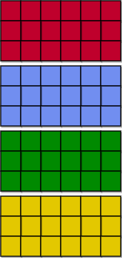
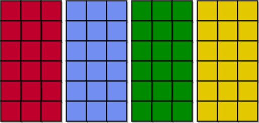
Consider the following.

How can we decompose the following problem?

Solution

Possible solutions include:

Consider the following.

How can we decompose the following problem?

Figure from Lee-Rausch, Beth. Application 53. 3D Domain Decomposition. NASA FUN3D: Fully Unstructured Navier-Stokes. July 2024. https://fun3d.larc.nasa.gov/example-53.html.

Some problems require irregular decomposition. There can be multiple reasons for this. One being that some portions of the problem requires more or less calculations. In other words, because of workloads. Another could be that some aspects of the problem require different calculations.

Key Points

Problem decomposition is problem dependent.

Utilize problem decomposition to boost parallel efficiency. Sometimes this requires irregular partitions.

previous episode

DeapSECURE module 6: Parallel and High-Performance Programming

next episode

Problem Decomposition

Overview