Tuning Neural Network Models for Better Accuracy
Overview
Teaching: 15 min
Exercises: 50 minQuestions
What is model tuning in Deep Learning?
What are the different types of tuning applicable to a neural network model?
What are the effects of tuning a particular hyperparameter to the performance of a model?
Is Jupyter notebook the best platform for such experiments?
Objectives
Tweak and tune deep learning models to obtain optimal performance.
Understand the effect of tuning the different hyperparameters.
Acquiring the art and common sense of the hyperparameter tuning.
Convert Python codes in a Jupyter notebook to a script and submit the script to HPC using a job scheduler.
Introduction
In the previous episode, we successfully built and trained a few neural network (NN) models to distinguish 18 running apps in an Android phone. We tested a model without hidden layer, as well as a model with one hidden layer. We saw a significant improvement of accuracy by adding just one hidden layer. This poses an interesting question: What is the limit of NN models in achieving the highest accuracy (or a similar performance metric)? We can intuitively speculate that adding more layers into the model would result in better and better accuracy. We can continue this refinement by constructing models with two, three, four hidden layers, and so on and so forth. The number of combinations will explode quickly, as each layer may also be varied in the number of hidden neurons. Every modified model must be retrained, which will make the entire process prohibitively expensive. We inevitably would have to stop the refinement at a certain point. All these testings are part of model tuning, an iterative process of refining an NN model so that it yields the best performance for the given task (such as smartphone app classification, in our case). In the model tuning process, we iteratively modify the NN model hyperparameters to find one model that has the most optimal performance.
In this episode, we will present a typical scenario for tuning an NN model. Consider the case of 18-apps classification task again: All the models have 19 input and 18 output nodes. The hidden layers of the model can be greatly varied, for example:
- A model with no hidden layer
- A model with one hidden layer of 18 neurons
- A model with two hidden layers of 18 neurons each
- A model with two hidden layers of 36 and 18 neurons, respectively
- … and many more!
The following hyperparameters in a model can be adjusted to find the best-performing NN model:
- the number of hidden layers (i.e. the depth of the network)
- the number of neurons per hidden layer (the width of the layer)
Collectively, the size of network inputs and outputs, plus the number of hidden layers and the number of neurons on each hidden layer, determine the architecture of an NN model.
The learning rate and batch size can also be adjusted. Although they are not part of the network architecture per se, they may affect the final accuracy of the model. So it is also important to find the optimal values for these hyperparameters as well.
Basic Procedure of Neural Network Model Tuning
The tuning process involves scanning the hyperparameter space, re-training the newly modified network and evaluate the model performance. A basic recipe for NN model tuning involves the following steps:
-
First, define the hyperparameter space we want to scan (e.g. the number of hidden layers = 1, 2, 3, …; the number of hidden neurons = 25, 50, 75, …).
-
Define (build) a new NN model with a specified hyperparameter setting (number of hidden layers, number of neurons in each layer, learning rate, batch size, …).
-
Train and validate the new model. From this process, we will want to compute and save the performance metrics of this model (i.e., one or more of: accuracy, precision, recall, etc.).
-
Repeat steps 1 and 2 until all the configurations we want to test have been tested. As you may anticipate, we will have to do a lot of trainings (at least one training per model).
-
Once we obtain all the performance metrics from each model, we will analyze these results to decide the most optimal NN model hyperparameter setting to achieve the best performance.
The following diagram shows the cycle of NN model tuning:
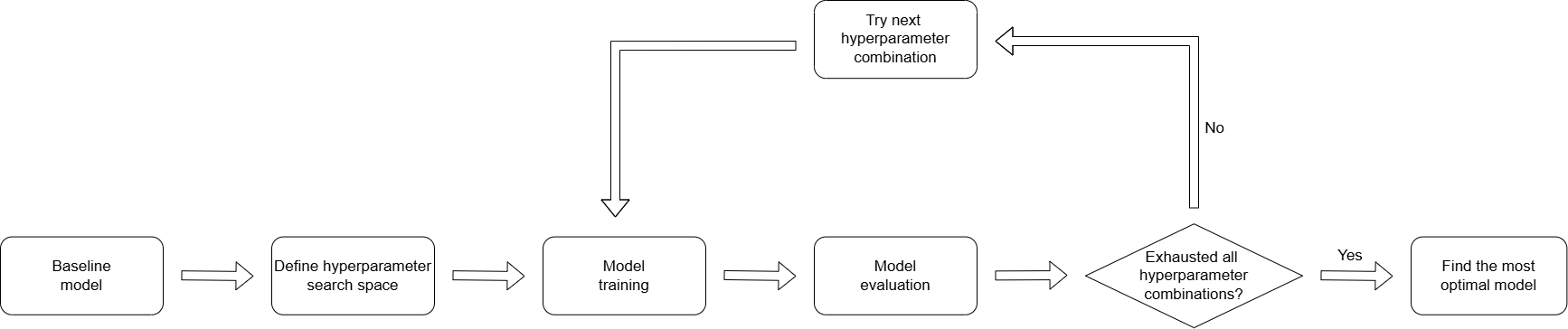
The optimal configuration is determined by the trade-off of the maximally achieveable accuracy versus the computational cost of training even more complex NN models.
Preparing Python Environment & the Dataset
Before diving into the model tuning experiments,
let us prepare our Python environment in the same way as in previous episode,
then load and preprocess the sherlock_18apps data.
(If you have just completed
the previous episode on NN modeling for the sherlock_18apps dataset
within the same interactive Python/Jupyter session
that will be used for this hands-on activity,
you do not need to perform this step.)
Loading Libraries &
sherlock_18appsDatasetFirst, load the Python libraries and the
sherlock_18appsdataset by running the commands in thePrep_ML.pyscript. In your current Jupyter session, use the magic command%loadto run the data preparation script:%load Prep_ML.pyPress Shift+Enter to execute this command; the contents of the script will be loaded into the active cell. Once loaded, press Shift+Enter once more to execute all the Python commands read from
Prep_ML.pyand get your environment ready. Please refer to “Data Preprocessing and Cleaning: A Review” section on the previous episode for the contents ofPrep_ML.pyand the expected outcome.As the last step, do remember to do one-hot encoding for the labels (
Prep_ML.pyalready takes care of one-hot encoding in the feature matrix):train_L_onehot = pd.get_dummies(train_labels) test_L_onehot = pd.get_dummies(test_labels)Next, load the TensorFlow, Keras, and visualization libraries:
# Import libraries
import tensorflow as tf
import tensorflow.keras as keras

from tensorflow.keras.models import Sequential
from tensorflow.keras.layers import Dense
from tensorflow.keras import optimizers
from tensorflow.keras.model import save_model, load_model

import matplotlib.pyplot as plt
Python Library: Gathering Useful Tools into a Toolbox
Programming Challenge: Writing a Function for Data Preprocessing
From this point, we will program in Python more intensively as we need to repeat many computations that are very similar (or identical) in nature. As the first case, we have repeated the data preparation above, which was first used in the previous episode.
Many parts of the program written above.
Instead of calling the Prep_ML.py file everytime we want to preprocess the dataset, we can create a function that performs the preprocessing for us. We can save this function to a file called
ML_toolbox.py, so it can be imported for easy use.def prep_ml(df): """ToDo: Summarize the dataset""" """ToDo: Delete irrelevant features and missing or bad data""" """ToDo: Separate labels from features""" """ToDo: Perform one-hot encoding for **all** categorical features.""" """ToDo: Feature scaling using StandardScaler.""" """ToDo: Perform train-test split on the master dataset.""" return train_features, test_features, train_labels, test_labelsTo test the function, create a new script that imports ML_toolbox.py, run the function, and then print out the return values.
The Baseline Model
Let us start by building a simple neural network model with one hidden layer. This will serve as a baseline model, which we will attempt to improve through the tuning process below:
def NN_Model_1H(hidden_neurons, learning_rate):
    """Definition of deep learning model with one dense hidden layer"""
    model = Sequential([
        # More hidden layers can be added here
        Dense(hidden_neurons, activation='relu', input_shape=(19,),
              kernel_initializer='random_normal'), # Hidden Layer
        Dense(18, activation='softmax',
              kernel_initializer='random_normal')  # Output Layer
    ])
    adam_opt = Adam(lr=learning_rate, beta_1=0.9, beta_2=0.999, amsgrad=False)
    model.compile(optimizer=adam_opt,
                  loss='categorical_crossentropy',
                  metrics=['accuracy'])
    return model
Reasoning for the Baseline Model
Why do we use a model with one hidden layer as a baseline, instead of the model with no hidden layer? Discuss this with your peer.
Solutions
We usually want to start with a fairly reasonable model as the baseline for tuning. The no-hidden-layer model has no hidden neurons by definition, so it lacks an important hyperparameter. Therefore the model’s usefulness as a baseline will be limited. We therefore use the one-hidden-layer model as our baseline.
More specifically, the baseline neural network model will have 18 neurons in the hidden layer. It will be trained with Adam optimizer with learning rate of 0.0003, batch size of 32, and epoch of 10. Let us construct and train this model:
model_1H = NN_Model_1H(18,0.0003)
model_1H_history = model_1H.fit(train_features,
                                train_L_onehot,
                                epochs=10, batch_size=32,
                                validation_data=(test_features, test_L_onehot),
                                verbose=2)
Epoch 1/10
6827/6827 - 10s - loss: 1.1037 - accuracy: 0.6752 - val_loss: 0.5488 - val_accuracy: 0.8702
Epoch 2/10
6827/6827 - 9s - loss: 0.4071 - accuracy: 0.9047 - val_loss: 0.3205 - val_accuracy: 0.9245
Epoch 3/10
6827/6827 - 9s - loss: 0.2743 - accuracy: 0.9319 - val_loss: 0.2425 - val_accuracy: 0.9385
Epoch 4/10
6827/6827 - 9s - loss: 0.2177 - accuracy: 0.9468 - val_loss: 0.1990 - val_accuracy: 0.9509
Epoch 5/10
6827/6827 - 9s - loss: 0.1818 - accuracy: 0.9592 - val_loss: 0.1692 - val_accuracy: 0.9628
Epoch 6/10
6827/6827 - 7s - loss: 0.1561 - accuracy: 0.9664 - val_loss: 0.1470 - val_accuracy: 0.9671
Epoch 7/10
6827/6827 - 9s - loss: 0.1363 - accuracy: 0.9703 - val_loss: 0.1296 - val_accuracy: 0.9708
Epoch 8/10
6827/6827 - 9s - loss: 0.1209 - accuracy: 0.9740 - val_loss: 0.1171 - val_accuracy: 0.9739
Epoch 9/10
6827/6827 - 9s - loss: 0.1089 - accuracy: 0.9769 - val_loss: 0.1058 - val_accuracy: 0.9770
Epoch 10/10
6827/6827 - 7s - loss: 0.0995 - accuracy: 0.9786 - val_loss: 0.0970 - val_accuracy: 0.9792
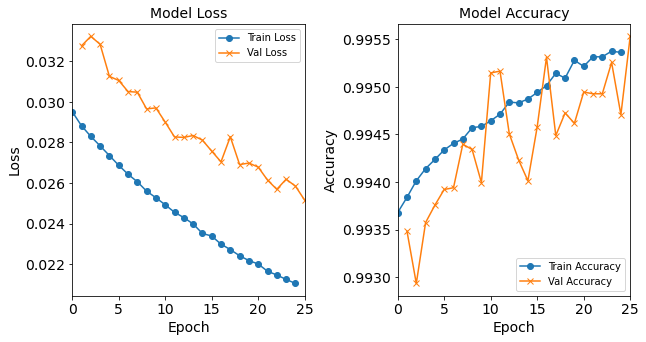
Let us visualize the model training history by borrowing the following functions from the previous episode.
plot_loss and plot_acc functions are designed to individually
plot the training and validation loss (plot_loss) and accuracy (plot_acc).
They take the model’s training history, an optional epoch shift to align x-axis epochs,
and a flag to show the plot immediately or not.
combine_plots function combines the insights from both loss and accuracy,
this function arranges them into a single, neatly organized figure with two subplots
– one for loss, another for accuracy.
It provides granular control over figure dimensions, subplot spacing,
and whether to individually display the subplots or show them all together in the end.
More details about the above functions can be found in the comments of the code.
Plotting Functions
plot_loss
# Function to plot the training and validation loss over epochs
def plot_loss(model_history, epoch_shifts= None, show=True):
    # If no epoch shifts are provided, default to (0,0)
    if epoch_shifts is None:
        epoch_shifts = (0, 0)

    # Calculate the shifted epochs for both training and validation
    epochs_train = np.array(model_history.epoch) + epoch_shifts[0]
    epochs_val = np.array(model_history.epoch) + epoch_shifts[1]

    # Plot training loss with circle markers
    plt.plot(epochs_train, model_history.history['loss'], '-o', label='Train Loss')
    # Plot validation loss with cross markers
    plt.plot(epochs_val, model_history.history['val_loss'], '-x', label='Val Loss')

    # Set plot title and axis labels
    plt.title('Model Loss', fontsize=14)
    plt.ylabel('Loss', fontsize=14)
    plt.xlabel('Epoch', fontsize=14)

    # Adjust x-axis limits to include all epochs
    plt.xlim([min(np.min(epochs_train), np.min(epochs_val)), max(np.max(epochs_train), np.max(epochs_val))])

    # Position the legend in the upper right corner
    plt.legend(loc='upper right')

    # Increase font size for axis ticks
    plt.tick_params(axis='x', labelsize=14)
    plt.tick_params(axis='y', labelsize=14)

    # Display the plot if 'show' is True
    if show:
        plt.show()

    # Return the current axis object for further manipulation if needed
    return plt.gca()
plot_acc
# Function to plot the training and validation accuracy over epochs
def plot_acc(model_history, epoch_shifts=None, show=True):
    # Default to (0,0) if no epoch shifts are provided
    if epoch_shifts is None:
        epoch_shifts = (0, 0)

    # Calculate the shifted epochs for both training and validation
    epochs_train = np.array(model_history.epoch) + epoch_shifts[0]
    epochs_val = np.array(model_history.epoch) + epoch_shifts[1]

    # Plot training accuracy with circle markers
    plt.plot(epochs_train, model_history.history['accuracy'], '-o', label='Train Accuracy')
    # Plot validation accuracy with cross markers
    plt.plot(epochs_val, model_history.history['val_accuracy'], '-x', label='Val Accuracy')

    # Set plot title and axis labels
    plt.title('Model Accuracy', fontsize=14)
    plt.ylabel('Accuracy', fontsize=14)
    plt.xlabel('Epoch', fontsize=14)

    # Adjust x-axis limits to include all epochs
    plt.xlim([min(np.min(epochs_train), np.min(epochs_val)), max(np.max(epochs_train), np.max(epochs_val))])

    # Position the legend in the lower right corner
    plt.legend(loc='lower right')

    # Increase font size for axis ticks
    plt.tick_params(axis='x', labelsize=14)
    plt.tick_params(axis='y', labelsize=14)

    # Display the plot if 'show' is True
    if show:
        plt.show()

    # Return the current axis object
    return plt.gca()
combine_plots
# Function to combine the loss and accuracy plots into a single figure with two subplots
def combine_plots(model_history,
                  plot_loss_func,
                  plot_acc_func,
                  figsize=(10.0, 5.0),
                  loss_epoch_shifts= None, loss_show=False,
                  acc_epoch_shifts= None, acc_show=False,  # Prevents immediate showing in subplots
                  wspace=0.4):  # Controls space between subplots

    # Create a new figure with the specified size
    plt.figure(figsize=figsize)

    # Subplot for loss
    plt.subplot(1, 2, 1)  # 1 row, 2 columns, first subplot
    plot_loss_func(model_history, epoch_shifts=loss_epoch_shifts, show=loss_show)  # Call plot_loss function

    # Subplot for accuracy
    plt.subplot(1, 2, 2)  # 1 row, 2 columns, second subplot
    plot_acc_func(model_history, epoch_shifts=acc_epoch_shifts, show=acc_show)  # Call plot_acc function

    # Adjust the space between subplots
    plt.subplots_adjust(wspace=wspace)

    # Finally, display the combined figure
    plt.show()
combine_plots(model_1H_history,
              plot_loss, plot_acc,
              loss_epoch_shifts=(0, 1), loss_show=False,
              acc_epoch_shifts=(0, 1), acc_show=False)
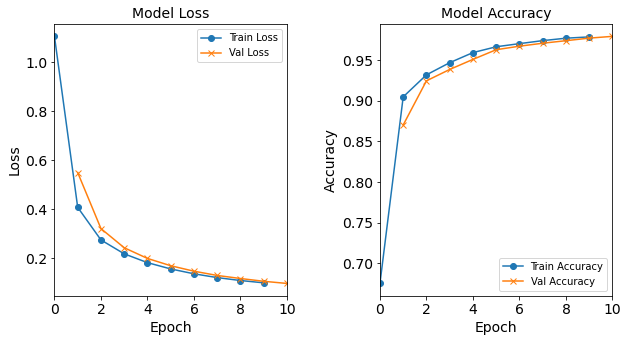
Before we attempt more sophisticated improvements, it is imperative to verify if our model training has converged. Here are several common methods for determining whether the model has converged:
- Keep training until the change in
loss(i.e., the loss value computed with the training set) oraccuracy(i.e., the proportion of correctly classified instances) between epochs N and N+1 is less than the predetermined threshold. - Monitoring the convergence curve
until the curve depicting
lossoraccuracytypically levels off or plateaus. This indicates that the model is no longer making significant improvements and has likely converged. - Set a suitable number of training epochs based on experience. Typically, the model will converge after this number of epochs.
Discuss the Training Convergence
In the training of
model_1Habove, please observe the changes inloss,val_loss,acc, andval_accas more epochs unfold.
- What are the changes in the earliest iterations (e.g. between epochs 1 and 2) and the latter iterations (e.g. between epochs 9 and 10)?
- How different are the values (and the changes in values) between those estimated from the training set (
lossandacc) and those from the validation set (val_lossandval_acc).- Has the model converged well enough with 10 epochs?
Solutions
The changes in the loss and accuracy at the beginning and ending of the training loops are as follows:
Between epochs change in losschange in accuracychange in val_losschange in val_accuracy1 –> 2 (beginning) -0.6966 0.2295 -0.2283 0.0543 9 –> 10 (ending) -0.0094 0.0017 -0.0088 0.0022 The changes in the loss and accuracy, for both training and validation datasets are dramatic at the beginning of the iteration. By the 10th iteration, the changes somewhat leveled off: the loss still decreases by about -0.009, and the accuracy still increases by about 0.2%.
In the second re-run of
fit(), the loss function has crossed over between the training and validation data. The accuracy of the train and test data are still tracking each other but with greater and greater apparent discrepancy; but we have to realize the changes in the accuracy between successive epochs are getting smaller and smaller.
Has this model converged? This is difficult to answer a priori (i.e. without prior knowledge). To determine whether our training has achieved good convergence, we should also consider this complementary question: What do you think is the limit of the accuracy of this model, before any tuning? Is this model capable only of 98% accuracy (which was achieved already by 10 epochs)? Can we reach 99%? How about 99.9%? Remember that in cybersecurity, we will really want to achieve as high an accuracy as possible to minimize wrong predictions. The best way to judge the convergence of the model is to run a few more training iterations, each time continuing from the previously trained model.
Checking Model Convergence: Train with More Epochs!
In order to continue the training on a model (model_1H in this case),
we simply call the fit function again on the model that has been previously trained.
You can decide the number of additional epochs to try.
For the second iteration below, we will train for 15 more epochs:
model_1H_history_p2 = model_1H.fit(train_features,
                                   train_L_onehot,
                                   epochs=15, batch_size=32,
                                   validation_data=(test_features, test_L_onehot),
                                   verbose=2)
Epoch 1/15
6827/6827 - 9s - loss: 0.0921 - accuracy: 0.9799 - val_loss: 0.0906 - val_accuracy: 0.9806
Epoch 2/15
6827/6827 - 9s - loss: 0.0860 - accuracy: 0.9811 - val_loss: 0.0854 - val_accuracy: 0.9821
Epoch 3/15
6827/6827 - 9s - loss: 0.0807 - accuracy: 0.9823 - val_loss: 0.0808 - val_accuracy: 0.9835
Epoch 4/15
6827/6827 - 9s - loss: 0.0761 - accuracy: 0.9840 - val_loss: 0.0760 - val_accuracy: 0.9838
Epoch 5/15
6827/6827 - 9s - loss: 0.0721 - accuracy: 0.9854 - val_loss: 0.0726 - val_accuracy: 0.9850
Epoch 6/15
6827/6827 - 9s - loss: 0.0688 - accuracy: 0.9866 - val_loss: 0.0694 - val_accuracy: 0.9849
Epoch 7/15
6827/6827 - 9s - loss: 0.0659 - accuracy: 0.9874 - val_loss: 0.0666 - val_accuracy: 0.9873
Epoch 8/15
6827/6827 - 9s - loss: 0.0633 - accuracy: 0.9880 - val_loss: 0.0650 - val_accuracy: 0.9867
Epoch 9/15
6827/6827 - 9s - loss: 0.0609 - accuracy: 0.9884 - val_loss: 0.0622 - val_accuracy: 0.9881
Epoch 10/15
6827/6827 - 9s - loss: 0.0588 - accuracy: 0.9887 - val_loss: 0.0597 - val_accuracy: 0.9886
Epoch 11/15
6827/6827 - 9s - loss: 0.0569 - accuracy: 0.9891 - val_loss: 0.0579 - val_accuracy: 0.9888
Epoch 12/15
6827/6827 - 9s - loss: 0.0551 - accuracy: 0.9891 - val_loss: 0.0563 - val_accuracy: 0.9890
Epoch 13/15
6827/6827 - 9s - loss: 0.0535 - accuracy: 0.9894 - val_loss: 0.0552 - val_accuracy: 0.9883
Epoch 14/15
6827/6827 - 9s - loss: 0.0519 - accuracy: 0.9895 - val_loss: 0.0539 - val_accuracy: 0.9888
Epoch 15/15
6827/6827 - 9s - loss: 0.0506 - accuracy: 0.9897 - val_loss: 0.0525 - val_accuracy: 0.9896
Since we are not tuning yet,
we must not change the values of the hyperparameters other than epochs.
The history from the second round of training is stored in model_1H_history_p2 object
(where p2 stands for “part 2”),
which we will need for plotting and analysis.
Reviewing the Second Training Round
Let us discuss the outcome of the second round of the training by answering the following questions:
At the end of the second call to the
fit()function, how many total epochs has this model been trained with?Compare the loss and accuracy of the model at the end of the first and second rounds of training. Additionally, what are the changes in the loss and accuracy at the end of the second round?
Estimate what would happen if we further train with more epochs?
Solutions
In our case above, after the second round of training, we have trained the model for a total of (10+15) = 25 epochs.
- At the end of the first round of training, we got an accuracy of nearly 98%, which still increased by about 0.2% between epoch 9 and 10. After the second round, the accuracy increased to almost 99% (a 1 percent improvement, which is not negligible!), and it was still increasing by less than 0.1%. Compare the following two outputs:
# the end of first fit() training: Epoch 10/10 6827/6827 - 12s - loss: 0.0996 - accuracy: 0.9785 - val_loss: 0.0970 - val_accuracy: 0.9792 # the end of second fit() training: Epoch 15/15 6827/6827 - 13s - loss: 0.0507 - accuracy: 0.9897 - val_loss: 0.0524 - val_accuracy: 0.9896- With further training, the accuracy can continue to improve, but at slower and slower rates.
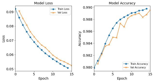
Plot the Progress of the Second Training Round
As a simple exercise, plot the progression of the loss function and accuracy in the second training round (hint: use the values in
model_1H_history_p2).Solutions
combine_plots(model_1H_history_p2,
              plot_loss, plot_acc,
              loss_epoch_shifts=(0, 1), loss_show=False,
              acc_epoch_shifts=(0, 1), acc_show=False)
For 3rd and 4th Rounds
Hint: You can run more training iterations as you see fit! In other words, the
model_0.fitcan be called many times; every time, it starts with the previously optimized model and further refines the parameters.The 3rd Round
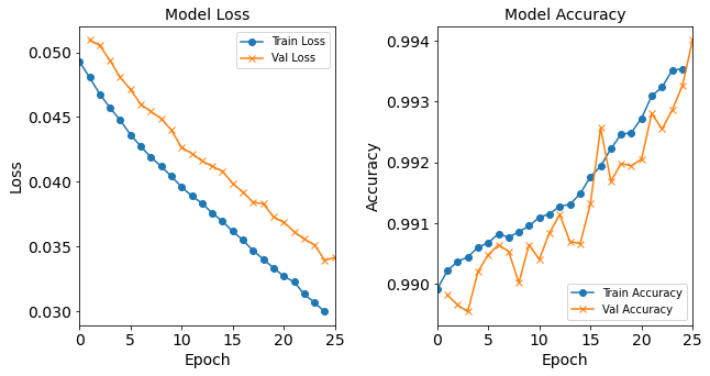
model_1H_history_p3 = model_1H.fit(train_features,
            train_L_onehot,
            epochs=25, batch_size=32,
            validation_data=(test_features, test_L_onehot),
            verbose=2)
Epoch 1/25 6827/6827 - 9s - loss: 0.0492 - accuracy: 0.9899 - val_loss: 0.0510 - val_accuracy: 0.9898 Epoch 2/25 6827/6827 - 9s - loss: 0.0480 - accuracy: 0.9902 - val_loss: 0.0506 - val_accuracy: 0.9897 Epoch 3/25 6827/6827 - 9s - loss: 0.0467 - accuracy: 0.9904 - val_loss: 0.0493 - val_accuracy: 0.9896 Epoch 4/25 6827/6827 - 9s - loss: 0.0456 - accuracy: 0.9905 - val_loss: 0.0478 - val_accuracy: 0.9903 Epoch 5/25 6827/6827 - 9s - loss: 0.0446 - accuracy: 0.9906 - val_loss: 0.0470 - val_accuracy: 0.9905 Epoch 6/25 6827/6827 - 9s - loss: 0.0436 - accuracy: 0.9907 - val_loss: 0.0460 - val_accuracy: 0.9906 Epoch 7/25 6827/6827 - 9s - loss: 0.0427 - accuracy: 0.9908 - val_loss: 0.0455 - val_accuracy: 0.9905 Epoch 8/25 6827/6827 - 9s - loss: 0.0419 - accuracy: 0.9908 - val_loss: 0.0449 - val_accuracy: 0.9900 Epoch 9/25 6827/6827 - 9s - loss: 0.0412 - accuracy: 0.9909 - val_loss: 0.0441 - val_accuracy: 0.9906 Epoch 10/25 6827/6827 - 9s - loss: 0.0404 - accuracy: 0.9910 - val_loss: 0.0428 - val_accuracy: 0.9904 Epoch 11/25 6827/6827 - 9s - loss: 0.0396 - accuracy: 0.9911 - val_loss: 0.0423 - val_accuracy: 0.9908 Epoch 12/25 6827/6827 - 9s - loss: 0.0389 - accuracy: 0.9912 - val_loss: 0.0417 - val_accuracy: 0.9912 Epoch 13/25 6827/6827 - 9s - loss: 0.0383 - accuracy: 0.9913 - val_loss: 0.0412 - val_accuracy: 0.9907 Epoch 14/25 6827/6827 - 9s - loss: 0.0375 - accuracy: 0.9913 - val_loss: 0.0408 - val_accuracy: 0.9907 Epoch 15/25 6827/6827 - 9s - loss: 0.0370 - accuracy: 0.9915 - val_loss: 0.0398 - val_accuracy: 0.9913 Epoch 16/25 6827/6827 - 9s - loss: 0.0361 - accuracy: 0.9918 - val_loss: 0.0391 - val_accuracy: 0.9926 Epoch 17/25 6827/6827 - 9s - loss: 0.0355 - accuracy: 0.9920 - val_loss: 0.0384 - val_accuracy: 0.9917 Epoch 18/25 6827/6827 - 9s - loss: 0.0347 - accuracy: 0.9923 - val_loss: 0.0382 - val_accuracy: 0.9920 Epoch 19/25 6827/6827 - 9s - loss: 0.0340 - accuracy: 0.9925 - val_loss: 0.0372 - val_accuracy: 0.9920 Epoch 20/25 6827/6827 - 9s - loss: 0.0333 - accuracy: 0.9925 - val_loss: 0.0367 - val_accuracy: 0.9921 Epoch 21/25 6827/6827 - 9s - loss: 0.0327 - accuracy: 0.9928 - val_loss: 0.0360 - val_accuracy: 0.9928 Epoch 22/25 6827/6827 - 9s - loss: 0.0320 - accuracy: 0.9931 - val_loss: 0.0354 - val_accuracy: 0.9925 Epoch 23/25 6827/6827 - 9s - loss: 0.0313 - accuracy: 0.9932 - val_loss: 0.0350 - val_accuracy: 0.9930 Epoch 24/25 6827/6827 - 9s - loss: 0.0306 - accuracy: 0.9935 - val_loss: 0.0336 - val_accuracy: 0.9933 Epoch 25/25 6827/6827 - 9s - loss: 0.0299 - accuracy: 0.9936 - val_loss: 0.0340 - val_accuracy: 0.9941combine_plots(model_1H_history_p3, plot_loss, plot_acc, loss_epoch_shifts=(0, 1), loss_show=False, acc_epoch_shifts=(0, 1), acc_show=False)
The 4th Round
model_1H_history_p4 = model_1H.fit(train_features,
            train_L_onehot,
            epochs=25, batch_size=32,
            validation_data=(test_features, test_L_onehot),
            verbose=2)
Epoch 1/25 6827/6827 - 9s - loss: 0.0294 - accuracy: 0.9937 - val_loss: 0.0326 - val_accuracy: 0.9935 Epoch 2/25 6827/6827 - 9s - loss: 0.0288 - accuracy: 0.9939 - val_loss: 0.0330 - val_accuracy: 0.9930 Epoch 3/25 6827/6827 - 9s - loss: 0.0283 - accuracy: 0.9940 - val_loss: 0.0328 - val_accuracy: 0.9936 Epoch 4/25 6827/6827 - 9s - loss: 0.0278 - accuracy: 0.9942 - val_loss: 0.0314 - val_accuracy: 0.9938 Epoch 5/25 6827/6827 - 9s - loss: 0.0273 - accuracy: 0.9943 - val_loss: 0.0311 - val_accuracy: 0.9939 Epoch 6/25 6827/6827 - 9s - loss: 0.0268 - accuracy: 0.9944 - val_loss: 0.0306 - val_accuracy: 0.9939 Epoch 7/25 6827/6827 - 9s - loss: 0.0264 - accuracy: 0.9944 - val_loss: 0.0304 - val_accuracy: 0.9944 Epoch 8/25 6827/6827 - 9s - loss: 0.0260 - accuracy: 0.9945 - val_loss: 0.0297 - val_accuracy: 0.9943 Epoch 9/25 6827/6827 - 9s - loss: 0.0256 - accuracy: 0.9946 - val_loss: 0.0300 - val_accuracy: 0.9940 Epoch 10/25 6827/6827 - 9s - loss: 0.0253 - accuracy: 0.9946 - val_loss: 0.0291 - val_accuracy: 0.9950 Epoch 11/25 6827/6827 - 9s - loss: 0.0249 - accuracy: 0.9946 - val_loss: 0.0283 - val_accuracy: 0.9952 Epoch 12/25 6827/6827 - 9s - loss: 0.0245 - accuracy: 0.9947 - val_loss: 0.0282 - val_accuracy: 0.9945 Epoch 13/25 6827/6827 - 9s - loss: 0.0244 - accuracy: 0.9948 - val_loss: 0.0282 - val_accuracy: 0.9942 Epoch 14/25 6827/6827 - 9s - loss: 0.0239 - accuracy: 0.9948 - val_loss: 0.0280 - val_accuracy: 0.9940 Epoch 15/25 6827/6827 - 9s - loss: 0.0235 - accuracy: 0.9949 - val_loss: 0.0276 - val_accuracy: 0.9945 Epoch 16/25 6827/6827 - 9s - loss: 0.0234 - accuracy: 0.9949 - val_loss: 0.0270 - val_accuracy: 0.9953 Epoch 17/25 6827/6827 - 9s - loss: 0.0230 - accuracy: 0.9950 - val_loss: 0.0285 - val_accuracy: 0.9945 Epoch 18/25 6827/6827 - 9s - loss: 0.0227 - accuracy: 0.9951 - val_loss: 0.0269 - val_accuracy: 0.9948 Epoch 19/25 6827/6827 - 9s - loss: 0.0226 - accuracy: 0.9951 - val_loss: 0.0270 - val_accuracy: 0.9946 Epoch 20/25 6827/6827 - 9s - loss: 0.0222 - accuracy: 0.9953 - val_loss: 0.0269 - val_accuracy: 0.9949 Epoch 21/25 6827/6827 - 9s - loss: 0.0220 - accuracy: 0.9952 - val_loss: 0.0261 - val_accuracy: 0.9949 Epoch 22/25 6827/6827 - 9s - loss: 0.0216 - accuracy: 0.9953 - val_loss: 0.0258 - val_accuracy: 0.9949 Epoch 23/25 6827/6827 - 9s - loss: 0.0215 - accuracy: 0.9954 - val_loss: 0.0261 - val_accuracy: 0.9952 Epoch 24/25 6827/6827 - 9s - loss: 0.0215 - accuracy: 0.9953 - val_loss: 0.0255 - val_accuracy: 0.9948 Epoch 25/25 6827/6827 - 9s - loss: 0.0210 - accuracy: 0.9954 - val_loss: 0.0250 - val_accuracy: 0.9956combine_plots(model_1H_history_p4, plot_loss, plot_acc, loss_epoch_shifts=(0, 1), loss_show=False, acc_epoch_shifts=(0, 1), acc_show=False)
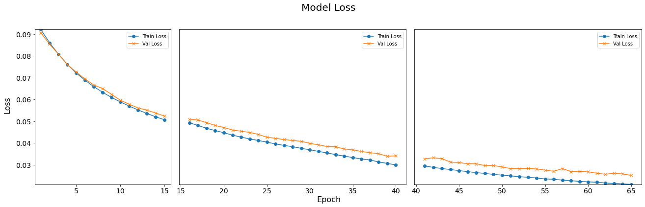
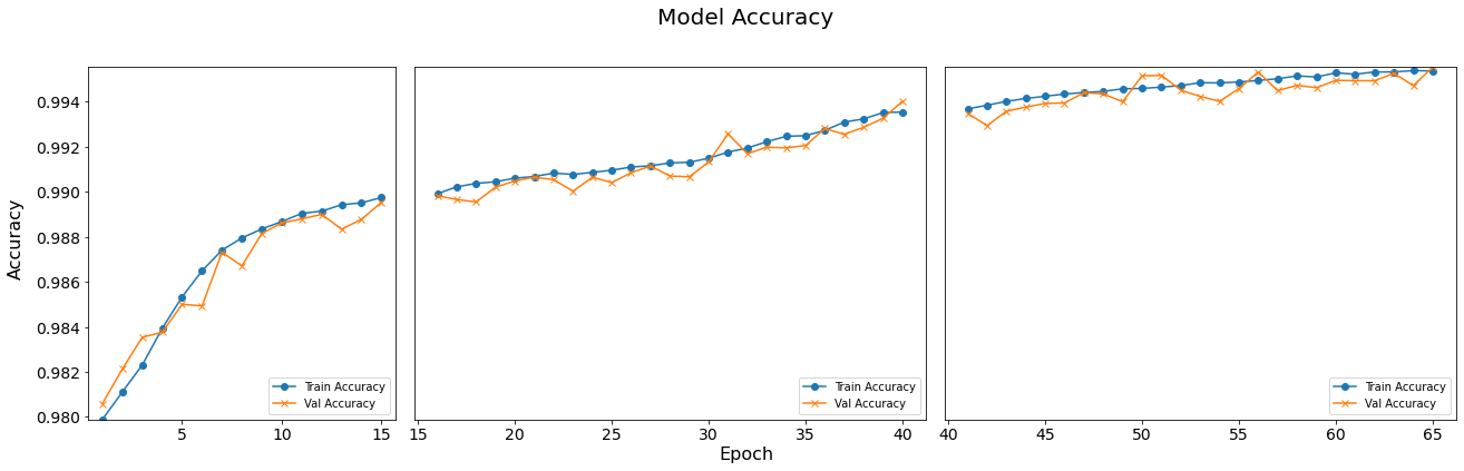
Consecutive Training Sessions
In above content, we’re examining the training progress of a model across multiple epochs. We’ve conducted three consecutive training sessions, each with additional epochs added, to observe how the model’s performance evolves over time. To visualize this progression more intuitively, we’ll plot the training loss and accuracy of each model side by side.
Three-subplot
Both plot_loss_subpanel and plot_accuracy_subpanel are designed to visualize the loss and accuracy of multiple models during training. Each function receives a list of model histories as input, which usually contains performance indicators of different models during training. The function creates a subgraph for each model and displays them side by side in the same chart to facilitate comparison of the performance of different models. More details can be found in the comments in the code.
def plot_loss_subpanel(model_histories):
   # Calculate epochs counts and determine width ratios for subplots
   epochs_counts = [len(history.history['loss']) for history in model_histories]
   total_epochs = sum(epochs_counts)
   width_ratios = [epochs / total_epochs for epochs in epochs_counts]

   # Initialize figure and grid layout
   fig = plt.figure(figsize=(20, 6))
   gs = gridspec.GridSpec(1, len(model_histories), width_ratios=width_ratios)

   # Initialize y-axis limits
   y_min, y_max = float('inf'), float('-inf')
   start_epoch = 0  # Start epoch counter for x-axis labeling

   # Loop through each model history
   for i, model_history in enumerate(model_histories):
       ax = fig.add_subplot(gs[i])  # Create subplot
       loss = model_history.history['loss']  # Training loss
       val_loss = model_history.history['val_loss']  # Validation loss
       epochs = range(start_epoch + 1, start_epoch + len(loss) + 1)  # Epochs range

       # Plot data with custom markers
       ax.plot(epochs, loss, '-o', label='Train Loss')
       ax.plot(epochs, val_loss, '-x', label='Val Loss')
       ax.legend(loc='upper right')  # Position legend

       # Update y-axis limit boundaries
       y_min = min(y_min, min(loss), min(val_loss))
       y_max = max(y_max, max(loss), max(val_loss))

       # Increment start_epoch for the next model's plot
       start_epoch += len(loss)

   # Apply uniform y-limits and adjust tick font sizes for all axes
   for ax in fig.get_axes():
       ax.set_ylim([y_min, y_max])
       ax.tick_params(axis='x', labelsize=14)
       ax.tick_params(axis='y', labelsize=14)

   # Hide y-axis labels and ticks for all but the first subplot
   for ax in fig.get_axes()[1:]:
       ax.set_yticklabels([])
       ax.set_yticks([])

   # Common x and y axis labels
   fig.text(0.5, 0.04, 'Epoch', ha='center', fontsize=16)
   fig.text(0.04, 0.5, 'Loss', va='center', rotation='vertical', fontsize=16)

   # Main title
   fig.suptitle('Model Loss', fontsize=20)

   # Adjust layout to fit well
   plt.tight_layout(rect=[0.05, 0.05, 0.95, 0.95])
   plt.show()  # Display the plot
def plot_accuracy_subpanel(model_histories): # Similar process as plot_loss_subpanel, adjusted for accuracy data epochs_counts = [len(history.history['accuracy']) for history in model_histories] total_epochs = sum(epochs_counts) width_ratios = [epochs / total_epochs for epochs in epochs_counts] fig = plt.figure(figsize=(20, 6)) gs = gridspec.GridSpec(1, len(model_histories), width_ratios=width_ratios) y_min, y_max = float('inf'), float('-inf') start_epoch = 0 for i, model_history in enumerate(model_histories): ax = fig.add_subplot(gs[i]) accuracy = model_history.history['accuracy'] val_accuracy = model_history.history['val_accuracy'] epochs = range(start_epoch + 1, start_epoch + len(accuracy) + 1) ax.plot(epochs, accuracy, '-o', label='Train Accuracy') ax.plot(epochs, val_accuracy, '-x', label='Val Accuracy') ax.legend(loc='lower right') # Legend at the bottom right y_min = min(y_min, min(accuracy), min(val_accuracy)) y_max = max(y_max, max(accuracy), max(val_accuracy)) start_epoch += len(accuracy) for ax in fig.get_axes(): ax.set_ylim([y_min, y_max]) ax.tick_params(axis='x', labelsize=14) ax.tick_params(axis='y', labelsize=14) for ax in fig.get_axes()[1:]: ax.set_yticklabels([]) ax.set_yticks([]) fig.text(0.5, 0.04, 'Epoch', ha='center', fontsize=16) fig.text(0.04, 0.5, 'Accuracy', va='center', rotation='vertical', fontsize=16) fig.suptitle('Model Accuracy', fontsize=20) plt.tight_layout(rect=[0.05, 0.05, 0.95, 0.95]) plt.show()plot_loss_subpanel([model_1H_history_p2, model_1H_history_p3, model_1H_history_p4]) plot_accuracy_subpanel([ model_1H_history_p2, model_1H_history_p3, model_1H_history_p4])
QUESTION:
What are other adjustable hyperparameters in this model?
Solutions
hidden_neurons(the number of neurons in the hidden layer),epochandbatch_sizeare three important hyperparameters. Activation function can also be considered a hyperparameter that affects the architecture of the model.
Model Tuning Experiments
Now that we have built and trained the baseline neural network model, we will run a variety of experiments using different combinations of hyperparameters, in order to find the best performing model. Below is a list of hyperparameters that could be interesting to explore; feel free to experiment with your own ideas as well.
We will use the NN_Model_1H with 18 neurons in the hidden layer as a baseline.
Starting from this model, let us:
- Test with different numbers of neurons in the hidden layer: 12, 8, 4, 2, 1
- It is also worthwhile to test a higher number of neurons: 40, 80, or more
- Test with different learning rates: 0.0003, 0.001, 0.01, 0.1
- Test with different batch sizes: 16, 32, 64, 128, 512, 1024
- Test with different numbers of hidden layers: 2, 3, and so on
NOTE: The easiest way to do this exploration is to simply copy the code cell where we constructed and trained the baseline model and paste it to a new cell below, since most of the parameters (
hidden_neurons,learning_rate,batch_size, etc.) can be changed when calling theNN_Model_1Hfunction or when fitting the model. However, to change the number of hidden layers (which we will do much later), the originalNN_model_1Hfunction must be duplicated and modified.
Tuning Experiments, Part 1: Varying Number of Neurons in Hidden Layers
In this round of experiments, we create several variants of NN_Model_1H models
with varying the hidden_neurons hyperparameter,
i.e. the number of neurons in the hidden layer.
The loss and accuracy of each model will be assessed as a function of hidden_neurons.
All the other hyperparameters (e.g. learning rate, epochs, batch_size, number of hidden layers)
will be kept constant; they will be varied later.
Not every number of hidden neurons is tested,
so feel free to create new code cells with a different number of neurons as your curiousity leads you.
Going in FEWER hidden neurons (vs input/output layers)
Model “1H12N”: 12 neurons in the hidden layer
#RUNIT
# the model with 12 neurons in the hidden layer
model_1H12N = NN_Model_1H(12,0.0003)
model_1H12N_history = model_1H12N.fit(train_features,
                                      train_L_onehot,
                                      epochs=10, batch_size=32,
                                      validation_data=(test_features, test_L_onehot),
                                      verbose=2)
combine_plots(model_1H12N_history,
              plot_loss, plot_acc,
              loss_epoch_shifts=(0, 1), loss_show=False,
              acc_epoch_shifts=(0, 1), acc_show=False)
Epoch 1/10
6827/6827 - 8s - loss: 1.1864 - accuracy: 0.6581 - val_loss: 0.6118 - val_accuracy: 0.8622
Epoch 2/10
6827/6827 - 9s - loss: 0.4592 - accuracy: 0.8992 - val_loss: 0.3700 - val_accuracy: 0.9217
Epoch 3/10
6827/6827 - 7s - loss: 0.3286 - accuracy: 0.9277 - val_loss: 0.2997 - val_accuracy: 0.9331
Epoch 4/10
6827/6827 - 7s - loss: 0.2803 - accuracy: 0.9349 - val_loss: 0.2659 - val_accuracy: 0.9381
Epoch 5/10
6827/6827 - 7s - loss: 0.2531 - accuracy: 0.9381 - val_loss: 0.2437 - val_accuracy: 0.9407
Epoch 6/10
6827/6827 - 9s - loss: 0.2328 - accuracy: 0.9413 - val_loss: 0.2253 - val_accuracy: 0.9448
Epoch 7/10
6827/6827 - 7s - loss: 0.2161 - accuracy: 0.9455 - val_loss: 0.2105 - val_accuracy: 0.9507
Epoch 8/10
6827/6827 - 7s - loss: 0.2026 - accuracy: 0.9496 - val_loss: 0.1983 - val_accuracy: 0.9549
Epoch 9/10
6827/6827 - 7s - loss: 0.1908 - accuracy: 0.9540 - val_loss: 0.1871 - val_accuracy: 0.9556
Epoch 10/10
6827/6827 - 9s - loss: 0.1777 - accuracy: 0.9565 - val_loss: 0.1731 - val_accuracy: 0.9593

Model “1H8N”: 8 neurons in the hidden layer
#RUNIT
model_1H8N = NN_Model_1H(8,0.0003)
model_1H8N_history = model_1H8N.fit(train_features,
                                    train_L_onehot,
                                    epochs=10, batch_size=32,
                                    validation_data=(test_features, test_L_onehot),
                                    verbose=2)
combine_plots(model_1H8N_history,
              plot_loss, plot_acc,
              loss_epoch_shifts=(0, 1), loss_show=False,
              acc_epoch_shifts=(0, 1), acc_show=False)
Epoch 1/10
6827/6827 - 8s - loss: 1.4420 - accuracy: 0.5361 - val_loss: 0.9016 - val_accuracy: 0.7646
Epoch 2/10
6827/6827 - 7s - loss: 0.6984 - accuracy: 0.8269 - val_loss: 0.5523 - val_accuracy: 0.8674
Epoch 3/10
6827/6827 - 8s - loss: 0.4725 - accuracy: 0.8843 - val_loss: 0.4205 - val_accuracy: 0.8979
Epoch 4/10
6827/6827 - 7s - loss: 0.3848 - accuracy: 0.9112 - val_loss: 0.3640 - val_accuracy: 0.9167
Epoch 5/10
6827/6827 - 7s - loss: 0.3445 - accuracy: 0.9195 - val_loss: 0.3347 - val_accuracy: 0.9224
Epoch 6/10
6827/6827 - 7s - loss: 0.3217 - accuracy: 0.9235 - val_loss: 0.3158 - val_accuracy: 0.9258
Epoch 7/10
6827/6827 - 8s - loss: 0.3057 - accuracy: 0.9269 - val_loss: 0.3015 - val_accuracy: 0.9272
Epoch 8/10
6827/6827 - 7s - loss: 0.2935 - accuracy: 0.9302 - val_loss: 0.2909 - val_accuracy: 0.9323
Epoch 9/10
6827/6827 - 7s - loss: 0.2833 - accuracy: 0.9319 - val_loss: 0.2822 - val_accuracy: 0.9339
Epoch 10/10
6827/6827 - 7s - loss: 0.2747 - accuracy: 0.9341 - val_loss: 0.2734 - val_accuracy: 0.9362

Tips & Tricks for Experimental Runs
Do you see the systematic names of the model and history variables, etc.?
The variable called model_1H12N means “a model with one hidden layer (1H)
that has 12 neurons (12N)”.
The use of systematic names, albeit complicated,
will be very helpful in keeping track of different experiments.
For example, down below, we will have models with two hidden layers;
such a model can be denoted by a variable name such as model_2H18N12N, etc.
DISCUSSION QUESTIONS:
Why don’t we just name the variables model1, model2, model3, …?
What are the advantages and disadvantages of naming them with this schema?
Keeping track of experimental results:
At this stage, it may be helpful to keep track the final training accuracy (after 10 epochs)
for each model with a distinct hidden_neurons value.
You can use pen-and-paper, or build a spreadsheet with the following
values:
hidden_neurons |
val_accuracy |
|---|---|
| 1 | …. |
| … | …. |
| 18 | 0.9792 (example) |
| … | …. |
| 80 | …. |
Exercises
Create additional code cells to run models with 4, 2, 1 neurons in the hidden layer
Model “1H4N”: 4 neurons in the hidden layer
#RUNIT
model_1H4N = NN_Model_1H(4,0.0003)
model_1H4N_history = model_1H4N.fit(train_features,
                                    train_L_onehot,
                                    epochs=10, batch_size=32,
                                    validation_data=(test_features, test_L_onehot),
                                    verbose=2)
combine_plots(model_1H4N_history,
              plot_loss, plot_acc,
              loss_epoch_shifts=(0, 1), loss_show=False,
              acc_epoch_shifts=(0, 1), acc_show=False)
Epoch 1/10 6827/6827 - 8s - loss: 1.6787 - accuracy: 0.4199 - val_loss: 1.2247 - val_accuracy: 0.5768 Epoch 2/10 6827/6827 - 7s - loss: 1.0693 - accuracy: 0.6315 - val_loss: 0.9432 - val_accuracy: 0.6934 Epoch 3/10 6827/6827 - 8s - loss: 0.8440 - accuracy: 0.7524 - val_loss: 0.7699 - val_accuracy: 0.7884 Epoch 4/10 6827/6827 - 8s - loss: 0.7248 - accuracy: 0.7993 - val_loss: 0.6817 - val_accuracy: 0.8122 Epoch 5/10 6827/6827 - 8s - loss: 0.6571 - accuracy: 0.8325 - val_loss: 0.6291 - val_accuracy: 0.8449 Epoch 6/10 6827/6827 - 8s - loss: 0.6146 - accuracy: 0.8495 - val_loss: 0.5927 - val_accuracy: 0.8491 Epoch 7/10 6827/6827 - 8s - loss: 0.5846 - accuracy: 0.8541 - val_loss: 0.5679 - val_accuracy: 0.8601 Epoch 8/10 6827/6827 - 8s - loss: 0.5640 - accuracy: 0.8572 - val_loss: 0.5498 - val_accuracy: 0.8783 Epoch 9/10 6827/6827 - 8s - loss: 0.5483 - accuracy: 0.8659 - val_loss: 0.5352 - val_accuracy: 0.8762 Epoch 10/10 6827/6827 - 8s - loss: 0.5347 - accuracy: 0.8701 - val_loss: 0.5208 - val_accuracy: 0.8687
Model “1H2N”: 2 neurons in the hidden layer
#RUNIT
model_1H2N = NN_Model_1H(2,0.0003)
model_1H2N_history = model_1H2N.fit(train_features,
                                    train_L_onehot,
                                    epochs=10, batch_size=32,
                                    validation_data=(test_features, test_L_onehot),
                                    verbose=2)
combine_plots(model_1H2N_history,
              plot_loss, plot_acc,
              loss_epoch_shifts=(0, 1), loss_show=False,
              acc_epoch_shifts=(0, 1), acc_show=False)
Epoch 1/10 6827/6827 - 9s - loss: 2.1385 - accuracy: 0.2973 - val_loss: 1.8072 - val_accuracy: 0.3491 Epoch 2/10 6827/6827 - 7s - loss: 1.6945 - accuracy: 0.3901 - val_loss: 1.6147 - val_accuracy: 0.4122 Epoch 3/10 6827/6827 - 7s - loss: 1.5603 - accuracy: 0.4286 - val_loss: 1.5186 - val_accuracy: 0.4345 Epoch 4/10 6827/6827 - 7s - loss: 1.4834 - accuracy: 0.4416 - val_loss: 1.4552 - val_accuracy: 0.4462 Epoch 5/10 6827/6827 - 7s - loss: 1.4283 - accuracy: 0.4535 - val_loss: 1.4069 - val_accuracy: 0.4610 Epoch 6/10 6827/6827 - 7s - loss: 1.3843 - accuracy: 0.4677 - val_loss: 1.3668 - val_accuracy: 0.4711 Epoch 7/10 6827/6827 - 7s - loss: 1.3467 - accuracy: 0.4811 - val_loss: 1.3322 - val_accuracy: 0.4803 Epoch 8/10 6827/6827 - 7s - loss: 1.3153 - accuracy: 0.4931 - val_loss: 1.3039 - val_accuracy: 0.4937 Epoch 9/10 6827/6827 - 8s - loss: 1.2892 - accuracy: 0.5089 - val_loss: 1.2802 - val_accuracy: 0.5120 Epoch 10/10 6827/6827 - 7s - loss: 1.2678 - accuracy: 0.5205 - val_loss: 1.2608 - val_accuracy: 0.5241
Model “1H1N”: 1 neuron in the hidden layer
#RUNIT
model_1H1N = NN_Model_1H(1,0.0003)
model_1H1N_history = model_1H1N.fit(train_features,
                                    train_L_onehot,
                                    epochs=10, batch_size=32,
                                    validation_data=(test_features, test_L_onehot),
                                    verbose=2)
combine_plots(model_1H1N_history,
              plot_loss, plot_acc,
              loss_epoch_shifts=(0, 1), loss_show=False,
              acc_epoch_shifts=(0, 1), acc_show=False)
Epoch 1/10 6827/6827 - 8s - loss: 2.3351 - accuracy: 0.2485 - val_loss: 2.1355 - val_accuracy: 0.2752 Epoch 2/10 6827/6827 - 7s - loss: 2.0610 - accuracy: 0.2724 - val_loss: 2.0034 - val_accuracy: 0.2723 Epoch 3/10 6827/6827 - 7s - loss: 1.9741 - accuracy: 0.2745 - val_loss: 1.9494 - val_accuracy: 0.2825 Epoch 4/10 6827/6827 - 7s - loss: 1.9346 - accuracy: 0.2829 - val_loss: 1.9205 - val_accuracy: 0.2857 Epoch 5/10 6827/6827 - 7s - loss: 1.9118 - accuracy: 0.2885 - val_loss: 1.9036 - val_accuracy: 0.2934 Epoch 6/10 6827/6827 - 8s - loss: 1.8976 - accuracy: 0.2937 - val_loss: 1.8930 - val_accuracy: 0.3008 Epoch 7/10 6827/6827 - 7s - loss: 1.8883 - accuracy: 0.3000 - val_loss: 1.8856 - val_accuracy: 0.3009 Epoch 8/10 6827/6827 - 7s - loss: 1.8819 - accuracy: 0.3048 - val_loss: 1.8808 - val_accuracy: 0.3149 Epoch 9/10 6827/6827 - 7s - loss: 1.8774 - accuracy: 0.3097 - val_loss: 1.8772 - val_accuracy: 0.3114 Epoch 10/10 6827/6827 - 8s - loss: 1.8737 - accuracy: 0.3112 - val_loss: 1.8742 - val_accuracy: 0.3104


Going in the direction of MORE hidden neurons
Models “1H40N” & “1H80N”: 40 & 80 neurons in the hidden layer
Exercises
Create more code cells to run models with 40 and 80 neurons in the hidden layer. You are welcome to explore even higher numbers of hidden neurons. Observe carefully what happening!
Model “1H4N”: 4 neurons in the hidden layer
#RUNIT
model_1H40N = NN_Model_1H(40,0.0003)
model_1H40N_history = model_1H40N.fit(train_features,
                                      train_L_onehot,
                                      epochs=10, batch_size=32,
                                      validation_data=(test_features, test_L_onehot),
                                      verbose=2)
combine_plots(model_1H40N_history,
              plot_loss, plot_acc,
              loss_epoch_shifts=(0, 1), loss_show=False,
              acc_epoch_shifts=(0, 1), acc_show=False)
Epoch 1/10 6827/6827 - 9s - loss: 0.8427 - accuracy: 0.7706 - val_loss: 0.3632 - val_accuracy: 0.9180 Epoch 2/10 6827/6827 - 9s - loss: 0.2798 - accuracy: 0.9339 - val_loss: 0.2265 - val_accuracy: 0.9456 Epoch 3/10 6827/6827 - 9s - loss: 0.1958 - accuracy: 0.9533 - val_loss: 0.1706 - val_accuracy: 0.9637 Epoch 4/10 6827/6827 - 9s - loss: 0.1519 - accuracy: 0.9658 - val_loss: 0.1364 - val_accuracy: 0.9689 Epoch 5/10 6827/6827 - 9s - loss: 0.1226 - accuracy: 0.9718 - val_loss: 0.1113 - val_accuracy: 0.9733 Epoch 6/10 6827/6827 - 9s - loss: 0.1014 - accuracy: 0.9770 - val_loss: 0.0931 - val_accuracy: 0.9796 Epoch 7/10 6827/6827 - 9s - loss: 0.0864 - accuracy: 0.9805 - val_loss: 0.0810 - val_accuracy: 0.9815 Epoch 8/10 6827/6827 - 9s - loss: 0.0755 - accuracy: 0.9825 - val_loss: 0.0704 - val_accuracy: 0.9822 Epoch 9/10 6827/6827 - 9s - loss: 0.0667 - accuracy: 0.9848 - val_loss: 0.0632 - val_accuracy: 0.9874 Epoch 10/10 6827/6827 - 9s - loss: 0.0596 - accuracy: 0.9875 - val_loss: 0.0570 - val_accuracy: 0.9884
Model “1H80N”: 80 neurons in the hidden layer
#RUNIT
model_1H80N = NN_Model_1H(80,0.0003)
model_1H80N_history = model_1H80N.fit(train_features,
                                      train_L_onehot,
                                      epochs=10, batch_size=32,
                                      validation_data=(test_features, test_L_onehot),
                                      verbose=2)
combine_plots(model_1H80N_history,
              plot_loss, plot_acc,
              loss_epoch_shifts=(0, 1), loss_show=False,
              acc_epoch_shifts=(0, 1), acc_show=False)
Epoch 1/10 6827/6827 - 9s - loss: 0.6815 - accuracy: 0.8244 - val_loss: 0.2710 - val_accuracy: 0.9327 Epoch 2/10 6827/6827 - 9s - loss: 0.2048 - accuracy: 0.9492 - val_loss: 0.1580 - val_accuracy: 0.9629 Epoch 3/10 >> 6827/6827 - 9s - loss: 0.1291 - accuracy: 0.9708 - val_loss: 0.1058 - val_accuracy: 0.9786 Epoch 4/10 6827/6827 - 9s - loss: 0.0900 - accuracy: 0.9808 - val_loss: 0.0764 - val_accuracy: 0.9829 Epoch 5/10 6827/6827 - 9s - loss: 0.0669 - accuracy: 0.9865 - val_loss: 0.0587 - val_accuracy: 0.9888 Epoch 6/10 6827/6827 - 9s - loss: 0.0525 - accuracy: 0.9902 - val_loss: 0.0463 - val_accuracy: 0.9915 Epoch 7/10 6827/6827 - 9s - loss: 0.0424 - accuracy: 0.9919 - val_loss: 0.0377 - val_accuracy: 0.9925 Epoch 8/10 6827/6827 - 9s - loss: 0.0351 - accuracy: 0.9931 - val_loss: 0.0326 - val_accuracy: 0.9933 Epoch 9/10 6827/6827 - 9s - loss: 0.0299 - accuracy: 0.9939 - val_loss: 0.0282 - val_accuracy: 0.9943 Epoch 10/10 6827/6827 - 9s - loss: 0.0258 - accuracy: 0.9945 - val_loss: 0.0244 - val_accuracy: 0.9948


Takeaways from Tuning Experiments Part 1
In the first experiment above, we tuned the NN_Model_1H model
by varying only the hidden_neurons hyperparameter.
CHALLENGE QUESTION
Please plot the final model accuracies against the number of hidden neurons.
Hint: you can do this in many ways! If you have kept track the accuracy vs.
hidden_neuronstable elsewhere, you can plot the results on a spreadsheet software (Google Sheets, Microsoft Excel, etc.). In this Python session, the final model accuracy can be found in the model history objects returned by thefit()function calls above. For example, the final accuracy from the model with 12 hidden neurons should be found inmodel_1H12N_history.history['val_accuracy'][-1](which should be close to 0.96)."""(Optional) Use this cell to generate the plot of val_acc vs. hidden_neurons:""" ## Example: # expt1_acc = [ # (1, model_1H1N_history['val_accuracy'][-1]), # # ... fill in the other values here # (12, model_1H12N_history['val_accuracy'][-1]), # # ... fill in the other values here # ] ## Construct a dataframe from expt1_acc # df_expt1_acc = pd.DataFrame(#TODO) ## Plot the data as an x-y line plot # df_expt1_acc.plot.line(#TODO)Solutions
#RUNIT

def get_val_acc(hist):
    return hist.history['val_accuracy'][-1]
#RUNIT expt1_acc = [ (1, get_val_acc(model_1H1N_history)), (2, get_val_acc(model_1H2N_history)), (4, get_val_acc(model_1H4N_history)), (8, get_val_acc(model_1H8N_history)), (12, get_val_acc(model_1H12N_history)), (18, get_val_acc(model_1H_history)), (40, get_val_acc(model_1H40N_history)), (80, get_val_acc(model_1H80N_history)), ]#RUNIT df_expt1_acc = pd.DataFrame(expt1_acc, columns=['hidden_neurons', 'val_accuracy']) df_expt1_acc
hidden_neurons val_accuracy 0 1 0.310367 1 2 0.524095 2 4 0.868701 3 8 0.936154 4 12 0.959279 5 18 0.979219 6 40 0.988447 7 80 0.994800 #RUNIT df_expt1_acc.plot.line(x='hidden_neurons', y='val_accuracy', style='o-') plt.title("Tuning Expt #1: Accuracy vs num of hidden neurons")

What Did We Learn from the Tuning Experiments Part 1?
Let us recap what we learned from this experiments by answering the following questions:
What happened to the model’s accuracy when we reduce
hidden_neurons? Describe the change in the accuracy of the model as we reducehidden_neuronsto an extremely small number.What happened to the accuracy if we increase
hidden_neurons? Discuss (or observe) what would happen if the hidden layer contains 1000 or even 10000 hidden neurons?In conclusion: In order to improve the accuracy of the model, should we use more or less hidden neurons?
Solutions
- When the number of hidden neurons in a model is reduced, a discernible trend begins to emerge in the accuracy of the model. Initially, a modest reduction in the hidden layer resulted in moderately worse accuracy. (A 2% reduction in the accuracy as we drop the number of hidden neurons from 18 to 12 is not negligible.) Reducing the number of hidden neurons to extremely low numbers leads to a significant damage in the model’s accuracy. This marked drop-off signifies that the model’s capacity to learn complex patterns and nuances within the data has been significantly curtailed. With too few neurons, the model becomes overly simplistic, unable to adequately represent the diversity and intricacies present in the dataset, leading to a substantial deterioration in predictive performance.
- TODO
In conclusion: While adding hidden neurons initially seems promising to improve accuracy, there is a point of diminishing returns beyond which accuracy may decrease due to overfitting or practical limitations. Finding the right balance in the number of hidden neurons is critical to achieving optimal model performance.
DISCUSSION:
What is an optimal value of
hidden_neuronsthat will yield the desirable level of accuracy? For example, what is the value ofhidden_neuronsthat will yield a 99% model accuracy? How about 99.5% accuracy? Can we reach 99.9% accuracy? Keep in mind that neural network model training is very expensive; increasing this hyperparameter may not improve the model significantly!
Deciding an Optimal Hyperparameter
The example above shows a common theme with model tuning.
The more neurons we train, the more accuracy we can achieve
(subject to risk of overfitting, see below).
You should have observed that at large enough hidden_neurons,
the model accuracy started to level off
(i.e. adding more neurons will not give significant gain in accuracy)?
Since training a neural network model is very expensive, we often have to make a trade-off between doing more trainings (which can be very costly, so may not be possible), and conserving effort against “point of diminishing return”, i.e. the point where improving the model does not yield a significant benefit in the model’s accuracy.
Where is the point of diminishing return?
This depends on the application. In some application we may really want to get as close as possible to 100%, then we have no choice but train more (bite the bullet).
Tuning Experiments, Part 2: Varying Learning Rate
In this batch of experiment, the accuracy and loss function of each model will be compared while changing the ‘learning rate’. For simplicity, all the other parameters (e.g. the number of neurons, epochs, batch_size, hidden layers) will be kept constant. The one hidden layer with 18 neurons model will be used. Not every number of learning rate is tested, so feel free to create new code cells with a different learning rate.
Model “1H18N” With Learning Rate 0.0003
model_1H18N_LR0_0003 = NN_Model_1H(18,0.0003)
model_1H18N_LR0_0003_history = model_1H18N_LR0_0003.fit(train_features,
                                                        train_L_onehot,
                                                        epochs=10, batch_size=32,
                                                        validation_data=(test_features, test_L_onehot),
                                                        verbose=2)

combine_plots(model_1H18N_LR0_0003_history,
              plot_loss, plot_acc,
              loss_epoch_shifts=(0, 1), loss_show=False,
              acc_epoch_shifts=(0, 1), acc_show=False)
Epoch 1/10
6827/6827 - 11s - loss: 1.1029 - accuracy: 0.6803 - val_loss: 0.5063 - val_accuracy: 0.8949
Epoch 2/10
6827/6827 - 10s - loss: 0.3616 - accuracy: 0.9233 - val_loss: 0.2791 - val_accuracy: 0.9413
Epoch 3/10
6827/6827 - 10s - loss: 0.2377 - accuracy: 0.9498 - val_loss: 0.2081 - val_accuracy: 0.9534
Epoch 4/10
6827/6827 - 10s - loss: 0.1850 - accuracy: 0.9585 - val_loss: 0.1678 - val_accuracy: 0.9620
Epoch 5/10
6827/6827 - 10s - loss: 0.1517 - accuracy: 0.9653 - val_loss: 0.1397 - val_accuracy: 0.9675
Epoch 6/10
6827/6827 - 10s - loss: 0.1287 - accuracy: 0.9705 - val_loss: 0.1209 - val_accuracy: 0.9725
Epoch 7/10
6827/6827 - 10s - loss: 0.1129 - accuracy: 0.9741 - val_loss: 0.1079 - val_accuracy: 0.9737
Epoch 8/10
6827/6827 - 10s - loss: 0.1016 - accuracy: 0.9758 - val_loss: 0.0982 - val_accuracy: 0.9770
Epoch 9/10
6827/6827 - 9s - loss: 0.0929 - accuracy: 0.9772 - val_loss: 0.0905 - val_accuracy: 0.9770
Epoch 10/10
6827/6827 - 10s - loss: 0.0859 - accuracy: 0.9787 - val_loss: 0.0847 - val_accuracy: 0.9788

Exercises
Create additional code cells to run models (
1H18N) with larger learning rates: 0.001, 0.01,0.1Model “1H18N” with Learning Rate 0.001
#RUNIT
model_1H18N_LR0_001 = NN_Model_1H(18,0.001)
model_1H18N_LR0_001_history = model_1H18N_LR0_001.fit(train_features,
                                      train_L_onehot,
                                      epochs=10, batch_size=32,
                                      validation_data=(test_features, test_L_onehot),
                                      verbose=2)

combine_plots(model_1H18N_LR0_001_history,
              plot_loss, plot_acc,
              loss_epoch_shifts=(0, 1), loss_show=False,
              acc_epoch_shifts=(0, 1), acc_show=False)
Epoch 1/10 6827/6827 - 10s - loss: 0.5687 - accuracy: 0.8485 - val_loss: 0.2241 - val_accuracy: 0.9488 Epoch 2/10 6827/6827 - 10s - loss: 0.1676 - accuracy: 0.9622 - val_loss: 0.1305 - val_accuracy: 0.9677 Epoch 3/10 6827/6827 - 10s - loss: 0.1106 - accuracy: 0.9740 - val_loss: 0.0954 - val_accuracy: 0.9750 Epoch 4/10 6827/6827 - 10s - loss: 0.0856 - accuracy: 0.9785 - val_loss: 0.0769 - val_accuracy: 0.9804 Epoch 5/10 6827/6827 - 10s - loss: 0.0712 - accuracy: 0.9827 - val_loss: 0.0656 - val_accuracy: 0.9829 Epoch 6/10 6827/6827 - 10s - loss: 0.0606 - accuracy: 0.9862 - val_loss: 0.0547 - val_accuracy: 0.9886 Epoch 7/10 6827/6827 - 10s - loss: 0.0522 - accuracy: 0.9884 - val_loss: 0.0505 - val_accuracy: 0.9893 Epoch 8/10 6827/6827 - 10s - loss: 0.0464 - accuracy: 0.9896 - val_loss: 0.0446 - val_accuracy: 0.9889 Epoch 9/10 6827/6827 - 10s - loss: 0.0416 - accuracy: 0.9904 - val_loss: 0.0393 - val_accuracy: 0.9909 Epoch 10/10 6827/6827 - 10s - loss: 0.0374 - accuracy: 0.9913 - val_loss: 0.0359 - val_accuracy: 0.9921
Model “1H18N” with Learning Rate 0.01
#RUNIT
model_1H18N_LR0_01 = NN_Model_1H(18,0.01)
model_1H18N_LR0_01_history = model_1H18N_LR0_01.fit(train_features,
                                      train_L_onehot,
                                      epochs=10, batch_size=32,
                                      validation_data=(test_features, test_L_onehot),
                                      verbose=2)
combine_plots(model_1H18N_LR0_01_history,
              plot_loss, plot_acc,
              loss_epoch_shifts=(0, 1), loss_show=False,
              acc_epoch_shifts=(0, 1), acc_show=False)
Epoch 1/10 6827/6827 - 10s - loss: 0.1858 - accuracy: 0.9505 - val_loss: 0.0807 - val_accuracy: 0.9772 Epoch 2/10 6827/6827 - 10s - loss: 0.0651 - accuracy: 0.9843 - val_loss: 0.0597 - val_accuracy: 0.9881 Epoch 3/10 6827/6827 - 10s - loss: 0.0494 - accuracy: 0.9882 - val_loss: 0.0434 - val_accuracy: 0.9884 Epoch 4/10 6827/6827 - 10s - loss: 0.0455 - accuracy: 0.9899 - val_loss: 0.0414 - val_accuracy: 0.9922 Epoch 5/10 6827/6827 - 10s - loss: 0.0426 - accuracy: 0.9905 - val_loss: 0.0357 - val_accuracy: 0.9927 Epoch 6/10 6827/6827 - 10s - loss: 0.0403 - accuracy: 0.9916 - val_loss: 0.0347 - val_accuracy: 0.9930 Epoch 7/10 6827/6827 - 10s - loss: 0.0322 - accuracy: 0.9925 - val_loss: 0.0406 - val_accuracy: 0.9902 Epoch 8/10 6827/6827 - 10s - loss: 0.0309 - accuracy: 0.9929 - val_loss: 0.0657 - val_accuracy: 0.9943 Epoch 9/10 6827/6827 - 13s - loss: 0.0301 - accuracy: 0.9936 - val_loss: 0.0326 - val_accuracy: 0.9960 Epoch 10/10 6827/6827 - 11s - loss: 0.0293 - accuracy: 0.9936 - val_loss: 0.0297 - val_accuracy: 0.9943
Model “1H18N” with Learning Rate 0.1
#RUNIT
model_1H18N_LR0_1 = NN_Model_1H(18,0.1)
model_1H18N_LR0_1_history = model_1H18N_LR0_1.fit(train_features,
                                      train_L_onehot,
                                      epochs=10, batch_size=32,
                                      validation_data=(test_features, test_L_onehot),
                                      verbose=2)
combine_plots(model_1H18N_LR0_1_history,
              plot_loss, plot_acc,
              loss_epoch_shifts=(0, 1), loss_show=False,
              acc_epoch_shifts=(0, 1), acc_show=False)
Epoch 1/10 6827/6827 - 10s - loss: 0.5033 - accuracy: 0.9238 - val_loss: 0.1934 - val_accuracy: 0.9453 Epoch 2/10 6827/6827 - 10s - loss: 0.3213 - accuracy: 0.9370 - val_loss: 0.4727 - val_accuracy: 0.9529 Epoch 3/10 6827/6827 - 10s - loss: 0.3065 - accuracy: 0.9402 - val_loss: 0.2525 - val_accuracy: 0.9428 Epoch 4/10 6827/6827 - 10s - loss: 0.3861 - accuracy: 0.9368 - val_loss: 0.3846 - val_accuracy: 0.9441 Epoch 5/10 6827/6827 - 10s - loss: 0.3262 - accuracy: 0.9367 - val_loss: 0.3117 - val_accuracy: 0.9498 Epoch 6/10 6827/6827 - 10s - loss: 0.4499 - accuracy: 0.9347 - val_loss: 0.3124 - val_accuracy: 0.9387 Epoch 7/10 6827/6827 - 10s - loss: 0.3448 - accuracy: 0.9374 - val_loss: 0.3204 - val_accuracy: 0.9432 Epoch 8/10 6827/6827 - 10s - loss: 0.3968 - accuracy: 0.9297 - val_loss: 0.2562 - val_accuracy: 0.9388 Epoch 9/10 6827/6827 - 10s - loss: 0.2790 - accuracy: 0.9315 - val_loss: 0.2671 - val_accuracy: 0.9276 Epoch 10/10 6827/6827 - 10s - loss: 0.3960 - accuracy: 0.9269 - val_loss: 0.2751 - val_accuracy: 0.9306


Takeaways from Tuning Experiments Part 2
In the second experiment above, we tuned the NN_Model_1H model
by varying the learning_rate hyperparameter.
CHALLENGE QUESTION
Please follow the method in the challenge question in tuning experiments part 1 to plot the relationship between the final model accuracy and different learning rates.
Solutions
expt2_acc = [
    (0.0003, get_acc(model_1H18N_LR0_0003_history)),
    (0.001, get_acc(model_1H18N_LR0_001_history)),
    (0.01, get_acc(model_1H18N_LR0_01_history)),
    (0.1, get_acc(model_1H18N_LR0_1_history))
]
#RUNIT df_expt2_acc = pd.DataFrame(expt2_acc, columns=['learning_rates', 'val_accuracy']) df_expt2_acc
learning_rates val_accuracy 0 0.0003 0.978797 1 0.0010 0.992090 2 0.0100 0.994287 3 0.1000 0.930643 #RUNIT df_expt2_acc.plot.line(x='learning_rates', y='val_accuracy', style='o-') plt.title("Tuning Expt #2: Accuracy vs learning rates")

What did we learn from the Tuning Experiments Part 2?
QUESTIONS:
Answer the questions below to recap what we learn about the effects of the learning rate.
1) What do you observe when we train the network with a small learning rate?
2) What happens to the training process when we increase the learning rate?
3) What happens to the training process when we increase the learning rate even further (to very large values)? Try a value of 0.1 or larger if you have not already.
4) What value of learning rate would you choose, and why?
ANSWERS:
1) When the learning rate is small, the updates to the weights and biases are small. This may cause the training process to converge slowly, requiring more iterations to achieve good results.
2) When the learning rate is large, the update magnitude of weights and biases increases, which can lead to faster training up to a certain value of learning rate.
3) Beyond this sweet spot, oscillations or instability may occur during training, or even failure to converge to a good solution. Learning rate of 0.01 seems to be good, but the validation accuracy shows an oscillation toward the latter epochs. Learning rates of 0.1 or larger are indeed not good.
4) Choosing an appropriate learning rate is one of the key factors when training a neural network, and it needs to be adjusted and optimized according to specific problems and experimental results.
Important Takeaway: Choosing an appropriate learning rate is one of the key factors when training a neural network, and it needs to be adjusted and optimized according to the specific problems and experimental results.
Tuning Experiments, Part 3: Varying Batch Size
The accuracy and loss of each model will be compared while changing the ‘batch size’. For simplicity, all other parameters (e.g. learning rate, epochs, number of neurons, hidden layers) will be kept constant. The one hidden layer with 18 neurons model will be used. Not every number of batch size is tested, so feel free to create new code cells with a different number of batch size.
model_1H18N_BS16 = NN_Model_1H(18,0.0003)
model_1H18N_BS16_history = model_1H18N_BS16.fit(train_features,
                                      train_L_onehot,
                                      epochs=10, batch_size=16,
                                      validation_data=(test_features, test_L_onehot),
                                      verbose=2)
combine_plots(model_1H18N_BS16_history,
              plot_loss, plot_acc,
              loss_epoch_shifts=(0, 1), loss_show=False,
              acc_epoch_shifts=(0, 1), acc_show=False)
Epoch 1/10
13654/13654 - 19s - loss: 0.8238 - accuracy: 0.7727 - val_loss: 0.3322 - val_accuracy: 0.9270
Epoch 2/10
13654/13654 - 19s - loss: 0.2556 - accuracy: 0.9388 - val_loss: 0.2078 - val_accuracy: 0.9495
Epoch 3/10
13654/13654 - 19s - loss: 0.1765 - accuracy: 0.9567 - val_loss: 0.1512 - val_accuracy: 0.9634
Epoch 4/10
13654/13654 - 18s - loss: 0.1350 - accuracy: 0.9688 - val_loss: 0.1210 - val_accuracy: 0.9720
Epoch 5/10
13654/13654 - 19s - loss: 0.1113 - accuracy: 0.9748 - val_loss: 0.1021 - val_accuracy: 0.9772
Epoch 6/10
13654/13654 - 19s - loss: 0.0962 - accuracy: 0.9792 - val_loss: 0.0899 - val_accuracy: 0.9812
Epoch 7/10
13654/13654 - 19s - loss: 0.0851 - accuracy: 0.9815 - val_loss: 0.0809 - val_accuracy: 0.9824
Epoch 8/10
13654/13654 - 19s - loss: 0.0767 - accuracy: 0.9829 - val_loss: 0.0734 - val_accuracy: 0.9826
Epoch 9/10
13654/13654 - 19s - loss: 0.0701 - accuracy: 0.9847 - val_loss: 0.0680 - val_accuracy: 0.9862
Epoch 10/10
13654/13654 - 19s - loss: 0.0647 - accuracy: 0.9862 - val_loss: 0.0639 - val_accuracy: 0.9836

Exercises
Create additional code cells to run models (
1H18N) with larger batch sizes, e.g. 16, 32, 64, 128, 512, 1024, …). Remember that we have the original batch_size=16.Model “1H18N” With Batch Size 32
#RUNIT
model_1H18N_BS32 = NN_Model_1H(18,0.0003)
model_1H18N_BS32_history = model_1H18N_BS32.fit(train_features,
                                      train_L_onehot,
                                      epochs=10, batch_size=32,
                                      validation_data=(test_features, test_L_onehot),
                                      verbose=2)
combine_plots(model_1H18N_BS32_history,
              plot_loss, plot_acc,
              loss_epoch_shifts=(0, 1), loss_show=False,
              acc_epoch_shifts=(0, 1), acc_show=False)
Epoch 1/10 6827/6827 - 10s - loss: 1.1029 - accuracy: 0.6803 - val_loss: 0.5063 - val_accuracy: 0.8949 Epoch 2/10 6827/6827 - 10s - loss: 0.3616 - accuracy: 0.9233 - val_loss: 0.2791 - val_accuracy: 0.9413 Epoch 3/10 6827/6827 - 10s - loss: 0.2377 - accuracy: 0.9498 - val_loss: 0.2081 - val_accuracy: 0.9534 Epoch 4/10 6827/6827 - 10s - loss: 0.1850 - accuracy: 0.9585 - val_loss: 0.1678 - val_accuracy: 0.9620 Epoch 5/10 6827/6827 - 10s - loss: 0.1517 - accuracy: 0.9653 - val_loss: 0.1397 - val_accuracy: 0.9675 Epoch 6/10 6827/6827 - 10s - loss: 0.1287 - accuracy: 0.9705 - val_loss: 0.1209 - val_accuracy: 0.9725 Epoch 7/10 6827/6827 - 10s - loss: 0.1129 - accuracy: 0.9741 - val_loss: 0.1079 - val_accuracy: 0.9737 Epoch 8/10 6827/6827 - 10s - loss: 0.1016 - accuracy: 0.9758 - val_loss: 0.0982 - val_accuracy: 0.9770 Epoch 9/10 6827/6827 - 10s - loss: 0.0929 - accuracy: 0.9772 - val_loss: 0.0905 - val_accuracy: 0.9770 Epoch 10/10 6827/6827 - 10s - loss: 0.0859 - accuracy: 0.9787 - val_loss: 0.0847 - val_accuracy: 0.9788
Model “1H18N” With Batch Size 64
#RUNIT
model_1H18N_BS64 = NN_Model_1H(18,0.0003)
model_1H18N_BS64_history = model_1H18N_BS64.fit(train_features,
                                      train_L_onehot,
                                      epochs=10, batch_size=64,
                                      validation_data=(test_features, test_L_onehot),
                                      verbose=2)
combine_plots(model_1H18N_BS64_history,
              plot_loss, plot_acc,
              loss_epoch_shifts=(0, 1), loss_show=False,
              acc_epoch_shifts=(0, 1), acc_show=False)
Epoch 1/10 3414/3414 - 6s - loss: 1.4388 - accuracy: 0.5565 - val_loss: 0.8041 - val_accuracy: 0.7991 Epoch 2/10 3414/3414 - 5s - loss: 0.5776 - accuracy: 0.8707 - val_loss: 0.4256 - val_accuracy: 0.9052 Epoch 3/10 3414/3414 - 5s - loss: 0.3546 - accuracy: 0.9216 - val_loss: 0.3060 - val_accuracy: 0.9325 Epoch 4/10 3414/3414 - 5s - loss: 0.2738 - accuracy: 0.9401 - val_loss: 0.2500 - val_accuracy: 0.9453 Epoch 5/10 3414/3414 - 5s - loss: 0.2294 - accuracy: 0.9504 - val_loss: 0.2141 - val_accuracy: 0.9519 Epoch 6/10 3414/3414 - 5s - loss: 0.1986 - accuracy: 0.9556 - val_loss: 0.1875 - val_accuracy: 0.9568 Epoch 7/10 3414/3414 - 5s - loss: 0.1750 - accuracy: 0.9597 - val_loss: 0.1665 - val_accuracy: 0.9613 Epoch 8/10 3414/3414 - 5s - loss: 0.1556 - accuracy: 0.9638 - val_loss: 0.1492 - val_accuracy: 0.9655 Epoch 9/10 3414/3414 - 5s - loss: 0.1399 - accuracy: 0.9671 - val_loss: 0.1350 - val_accuracy: 0.9674 Epoch 10/10 3414/3414 - 5s - loss: 0.1273 - accuracy: 0.9715 - val_loss: 0.1238 - val_accuracy: 0.9727
Model “1H18N” With Batch Size 128
#RUNIT
model_1H18N_BS128 = NN_Model_1H(18,0.0003)
model_1H18N_BS128_history = model_1H18N_BS128.fit(train_features,
                                      train_L_onehot,
                                      epochs=10, batch_size=128,
                                      validation_data=(test_features, test_L_onehot),
                                      verbose=2)
combine_plots(model_1H18N_BS128_history,
              plot_loss, plot_acc,
              loss_epoch_shifts=(0, 1), loss_show=False,
              acc_epoch_shifts=(0, 1), acc_show=False)
Epoch 1/10 1707/1707 - 4s - loss: 1.8142 - accuracy: 0.4222 - val_loss: 1.1781 - val_accuracy: 0.6165 Epoch 2/10 1707/1707 - 3s - loss: 0.9118 - accuracy: 0.7627 - val_loss: 0.7089 - val_accuracy: 0.8346 Epoch 3/10 1707/1707 - 3s - loss: 0.5814 - accuracy: 0.8680 - val_loss: 0.4835 - val_accuracy: 0.8870 Epoch 4/10 1707/1707 - 3s - loss: 0.4178 - accuracy: 0.8995 - val_loss: 0.3700 - val_accuracy: 0.9096 Epoch 5/10 1707/1707 - 3s - loss: 0.3344 - accuracy: 0.9209 - val_loss: 0.3081 - val_accuracy: 0.9280 Epoch 6/10 1707/1707 - 3s - loss: 0.2854 - accuracy: 0.9337 - val_loss: 0.2688 - val_accuracy: 0.9384 Epoch 7/10 1707/1707 - 3s - loss: 0.2521 - accuracy: 0.9426 - val_loss: 0.2398 - val_accuracy: 0.9471 Epoch 8/10 1707/1707 - 3s - loss: 0.2262 - accuracy: 0.9491 - val_loss: 0.2164 - val_accuracy: 0.9505 Epoch 9/10 1707/1707 - 3s - loss: 0.2052 - accuracy: 0.9528 - val_loss: 0.1972 - val_accuracy: 0.9536 Epoch 10/10 1707/1707 - 3s - loss: 0.1879 - accuracy: 0.9550 - val_loss: 0.1814 - val_accuracy: 0.9551
Model “1H18N” With Batch Size 512
#RUNIT
model_1H18N_BS512 = NN_Model_1H(18,0.0003)
model_1H18N_BS512_history = model_1H18N_BS512.fit(train_features,
                                      train_L_onehot,
                                      epochs=10, batch_size=512,
                                      validation_data=(test_features, test_L_onehot),
                                      verbose=2)
combine_plots(model_1H18N_BS512_history,
              plot_loss, plot_acc,
              loss_epoch_shifts=(0, 1), loss_show=False,
              acc_epoch_shifts=(0, 1), acc_show=False)
Epoch 1/10 427/427 - 1s - loss: 2.5478 - accuracy: 0.2648 - val_loss: 2.0955 - val_accuracy: 0.3152 Epoch 2/10 427/427 - 1s - loss: 1.8088 - accuracy: 0.4025 - val_loss: 1.5753 - val_accuracy: 0.4566 Epoch 3/10 427/427 - 1s - loss: 1.4084 - accuracy: 0.5331 - val_loss: 1.2653 - val_accuracy: 0.5890 Epoch 4/10 427/427 - 1s - loss: 1.1491 - accuracy: 0.6474 - val_loss: 1.0477 - val_accuracy: 0.6946 Epoch 5/10 427/427 - 1s - loss: 0.9598 - accuracy: 0.7376 - val_loss: 0.8844 - val_accuracy: 0.7828 Epoch 6/10 427/427 - 1s - loss: 0.8154 - accuracy: 0.8087 - val_loss: 0.7568 - val_accuracy: 0.8250 Epoch 7/10 427/427 - 1s - loss: 0.6995 - accuracy: 0.8407 - val_loss: 0.6515 - val_accuracy: 0.8484 Epoch 8/10 427/427 - 1s - loss: 0.6063 - accuracy: 0.8697 - val_loss: 0.5704 - val_accuracy: 0.8790 Epoch 9/10 427/427 - 1s - loss: 0.5349 - accuracy: 0.8828 - val_loss: 0.5077 - val_accuracy: 0.8848 Epoch 10/10 427/427 - 1s - loss: 0.4792 - accuracy: 0.8887 - val_loss: 0.4581 - val_accuracy: 0.8906
Model “1H18N” With Batch Size 1024
#RUNIT
model_1H18N_BS1024 = NN_Model_1H(18,0.0003)
model_1H18N_BS1024_history = model_1H18N_BS1024.fit(train_features,
                                      train_L_onehot,
                                      epochs=10, batch_size=1024,
                                      validation_data=(test_features, test_L_onehot),
                                      verbose=2)
combine_plots(model_1H18N_BS1024_history,
              plot_loss, plot_acc,
              loss_epoch_shifts=(0, 1), loss_show=False,
              acc_epoch_shifts=(0, 1), acc_show=False)
Epoch 1/10 214/214 - 1s - loss: 2.7688 - accuracy: 0.2434 - val_loss: 2.5636 - val_accuracy: 0.3167 Epoch 2/10 214/214 - 1s - loss: 2.3085 - accuracy: 0.3085 - val_loss: 2.0787 - val_accuracy: 0.3201 Epoch 3/10 214/214 - 1s - loss: 1.9158 - accuracy: 0.3856 - val_loss: 1.7679 - val_accuracy: 0.4188 Epoch 4/10 214/214 - 1s - loss: 1.6514 - accuracy: 0.4357 - val_loss: 1.5421 - val_accuracy: 0.4649 Epoch 5/10 214/214 - 1s - loss: 1.4515 - accuracy: 0.5100 - val_loss: 1.3691 - val_accuracy: 0.5613 Epoch 6/10 214/214 - 1s - loss: 1.2958 - accuracy: 0.5860 - val_loss: 1.2295 - val_accuracy: 0.6109 Epoch 7/10 214/214 - 1s - loss: 1.1667 - accuracy: 0.6487 - val_loss: 1.1110 - val_accuracy: 0.6735 Epoch 8/10 214/214 - 1s - loss: 1.0568 - accuracy: 0.6860 - val_loss: 1.0103 - val_accuracy: 0.7002 Epoch 9/10 214/214 - 1s - loss: 0.9632 - accuracy: 0.7167 - val_loss: 0.9237 - val_accuracy: 0.7638 Epoch 10/10 214/214 - 1s - loss: 0.8815 - accuracy: 0.7684 - val_loss: 0.8473 - val_accuracy: 0.8006


Takeaways from Tuning Experiments Part 3
In the third experiment above, we tuned the NN_Model_1H model
by varying the batch_size hyperparameter.
CHALLENGE QUESTION
Please follow the method in the challenge question in tuning experiments part 1 to plot the relationship between the final model accuracy and different batch sizes.
Solutions
expt3_acc = [
    (16, get_acc(model_1H18N_BS16_history)),
    (32, get_acc(model_1H18N_BS32_history)),
    (64, get_acc(model_1H18N_BS64_history)),
    (128, get_acc(model_1H18N_BS128_history)),
    (512, get_acc(model_1H18N_BS512_history)),
    (1024, get_acc(model_1H18N_BS1024_history))
]
#RUNIT df_expt3_acc = pd.DataFrame(expt3_acc, columns=['batch_sizes', 'val_accuracy']) df_expt3_acc
batch_sizes val_accuracy 0 16 0.983613 1 32 0.978797 2 64 0.972719 3 128 0.955123 4 512 0.890581 5 1024 0.800645 #RUNIT df_expt3_acc.plot.line(x='batch_sizes', y='val_accuracy', style='o-') plt.title("Tuning Expt #3: Accuracy vs batch sizes")

What did we learn from the Tuning Experiments Part 3?
QUESTIONS:
Answer the questions below to recap what we learn about the effects of the learning rate.
1) What do you observe when the batch size changes?
2) How to choose the right batch size?
ANSWERS:
1) As the batch size increases, although the training time is shortened, the accuracy rate decreases.
2) Common batch size choices are powers of 2 (e.g., 32, 64, 128, 256) due to hardware optimizations. However, there is no one-size-fits-all answer. It depends on the specific problem, dataset, model architecture, and available resources.
Tuning Experiments, Part 4: Varying the number of hidden layers
The accuracy and loss of each model will be compared while changing the ‘number of hidden layers’. For simplicity, all other parameters (e.g. learning rate, epochs, batch_size, number of neurons) will be kept constant. Not every number of hidden layers is tested, so feel free to create new code cells with a different number of layers.
def NN_Model_2H(hidden_neurons_1,sec_hidden_neurons_1, learning_rate):
    """Definition of deep learning model with one dense hidden layer"""
    model = Sequential([
        # More hidden layers can be added here
        Dense(hidden_neurons_1, activation='relu', input_shape=(19,),
              kernel_initializer='random_normal'), # Hidden Layer
        Dense(hidden_neurons_1, activation='relu',
              kernel_initializer='random_normal'), # Hidden Layer
        Dense(18, activation='softmax',
              kernel_initializer='random_normal')  # Output Layer
    ])
    adam_opt = Adam(lr=learning_rate, beta_1=0.9, beta_2=0.999, amsgrad=False)
    model.compile(optimizer=adam_opt,
                  loss='categorical_crossentropy',
                  metrics=['accuracy'])
    return model
#RUNIT
# the model with 18 neurons in the hidden layer
model_2H18N18N = NN_Model_2H(18,18,0.0003)
model_2H18N18N_history = model_2H18N18N.fit(train_features,
                                      train_L_onehot,
                                      epochs=10, batch_size=32,
                                      validation_data=(test_features, test_L_onehot),
                                      verbose=2)
combine_plots(model_2H18N18N_history,
              plot_loss, plot_acc,
              loss_epoch_shifts=(0, 1), loss_show=False,
              acc_epoch_shifts=(0, 1), acc_show=False)
Epoch 1/10
6827/6827 - 11s - loss: 1.0831 - accuracy: 0.6562 - val_loss: 0.4132 - val_accuracy: 0.8996
Epoch 2/10
6827/6827 - 10s - loss: 0.3015 - accuracy: 0.9291 - val_loss: 0.2294 - val_accuracy: 0.9455
Epoch 3/10
6827/6827 - 11s - loss: 0.1911 - accuracy: 0.9538 - val_loss: 0.1598 - val_accuracy: 0.9605
Epoch 4/10
6827/6827 - 10s - loss: 0.1413 - accuracy: 0.9648 - val_loss: 0.1254 - val_accuracy: 0.9696
Epoch 5/10
6827/6827 - 10s - loss: 0.1136 - accuracy: 0.9722 - val_loss: 0.1035 - val_accuracy: 0.9770
Epoch 6/10
6827/6827 - 10s - loss: 0.0941 - accuracy: 0.9776 - val_loss: 0.0871 - val_accuracy: 0.9800
Epoch 7/10
6827/6827 - 10s - loss: 0.0789 - accuracy: 0.9812 - val_loss: 0.0741 - val_accuracy: 0.9839
Epoch 8/10
6827/6827 - 10s - loss: 0.0661 - accuracy: 0.9846 - val_loss: 0.0615 - val_accuracy: 0.9862
Epoch 9/10
6827/6827 - 10s - loss: 0.0552 - accuracy: 0.9876 - val_loss: 0.0529 - val_accuracy: 0.9892
Epoch 10/10
6827/6827 - 10s - loss: 0.0476 - accuracy: 0.9899 - val_loss: 0.0476 - val_accuracy: 0.9892

Exercises
Create additional code cells to run models (
3H18N18N18N).Solutions
def NN_Model_3H(hidden_neurons_1,hidden_neurons_2, hidden_neurons_3, learning_rate):
    """Definition of deep learning model with one dense hidden layer"""
    model = Sequential([
        # More hidden layers can be added here
        Dense(hidden_neurons_1, activation='relu', input_shape=(19,),
              kernel_initializer='random_normal'), # Hidden Layer
        Dense(hidden_neurons_2, activation='relu',
              kernel_initializer='random_normal'), # Hidden Layer
        Dense(hidden_neurons_3, activation='relu',
              kernel_initializer='random_normal'), # Hidden Layer
        Dense(18, activation='softmax',
              kernel_initializer='random_normal')  # Output Layer
    ])
    adam_opt = Adam(lr=learning_rate, beta_1=0.9, beta_2=0.999, amsgrad=False)
    model.compile(optimizer=adam_opt,
                  loss='categorical_crossentropy',
                  metrics=['accuracy'])
    return model
#RUNIT model_3H18N18N18N = NN_Model_3H(18,18,18,0.0003) model_3H18N18N18N_history = model_3H18N18N18N.fit(train_features, train_L_onehot, epochs=10, batch_size=32, validation_data=(test_features, test_L_onehot), verbose=2) combine_plots(model_3H18N18N18N_history, plot_loss, plot_acc, loss_epoch_shifts=(0, 1), loss_show=False, acc_epoch_shifts=(0, 1), acc_show=False)Epoch 1/10 6827/6827 - 12s - loss: 1.1242 - accuracy: 0.6479 - val_loss: 0.5027 - val_accuracy: 0.8687 Epoch 2/10 6827/6827 - 12s - loss: 0.3823 - accuracy: 0.9136 - val_loss: 0.3072 - val_accuracy: 0.9347 Epoch 3/10 6827/6827 - 12s - loss: 0.2567 - accuracy: 0.9467 - val_loss: 0.2181 - val_accuracy: 0.9569 Epoch 4/10 6827/6827 - 11s - loss: 0.1887 - accuracy: 0.9587 - val_loss: 0.1631 - val_accuracy: 0.9622 Epoch 5/10 6827/6827 - 12s - loss: 0.1415 - accuracy: 0.9641 - val_loss: 0.1224 - val_accuracy: 0.9670 Epoch 6/10 6827/6827 - 12s - loss: 0.1097 - accuracy: 0.9725 - val_loss: 0.0974 - val_accuracy: 0.9765 Epoch 7/10 6827/6827 - 12s - loss: 0.0903 - accuracy: 0.9794 - val_loss: 0.0822 - val_accuracy: 0.9818 Epoch 8/10 6827/6827 - 12s - loss: 0.0783 - accuracy: 0.9826 - val_loss: 0.0730 - val_accuracy: 0.9839 Epoch 9/10 6827/6827 - 12s - loss: 0.0685 - accuracy: 0.9844 - val_loss: 0.0667 - val_accuracy: 0.9841 Epoch 10/10 6827/6827 - 12s - loss: 0.0615 - accuracy: 0.9858 - val_loss: 0.0595 - val_accuracy: 0.9833

What did we learn from the Tuning Experiments Part 4?
QUESTIONS:
Answer the questions below to recap what we learn about the effects of the number of hidden layers.
1) How many neurons to use in each hidden layer?
2) What did you observe?
3) What do we learn from here?
ANSWERS:
1) From the names of the models model_2H18N18N and model_3H18N18N18N, ‘ we can see that each hidden layer has 18 neurons.
2) * Compared to the more expensive network down below (3 hidden layers, @ 18 neurons each,0.9844), it seems like we can gain the similar accuracy with 1 hidden layer @ 18 neurons (~0.9811) We can gain the higher accuracy (~0.9882) with the network (2 hidden layers, @ 18 neurons each) than the network (3 hidden layers, @ 18 neurons each).
3) Usually, the more neurons we train, the more accuracy we can get (subject to risk of overfitting, vanishing and exploding gradients, see below)
While increasing the number of hidden layers in a neural network can potentially improve its ability to learn complex patterns and representations, it does not guarantee higher accuracy.
CHALLENGE QUESTION
(Optional, challenging) Try to vary the number of neurons in the hidden layers (add / subtract as needed) and check the results.
Additional Tuning Opportunities
There are other hyperparameters that can be adjusted:
- Change the optimizer (try optimizers other than
Adam) - Activation function (this is actually a part of the network’s architecture)
We encourage you to explore the effects of changing these in your network.
Summary
By going through this notebook it will be obvious that creating a deep learning experiment using the jupyter notebook will get messy and laborious. by the end of this notebook you will learn how to utilize scripting as well as using the power of HPC to alleviate the pain of executing block by block of jupyter notebook and make this experiment fast.
How was the experiment of model tuning so far? frustrating? confusing? So, let’s be honest, any machine learning experiment is going to have some level of uncertainty when dealing with unseen data. Especially when you don’t know how your model will respond to your features. This makes the model tuning process a must process!. In this notebook, by learning about different neural networks hyperparameters and tunning some of them including hidden layers, hidden neurons, learning rate, etc., we tried to monitor the effects on timing and accuracy. These timing and accuracy results were also visualized graphically and saved to csv format for later.
Now, I want to shift your attention from the model tuning process to the platform in which we did our experiment. The jupyter notebook is an excellent platform to create code, experiment on and get the results. but I don’t know about you but for me, the single cell to single cell execution of commands seems tedious. In the beginning of this notebook I have touched on how doing experiments like we did so far can get messy in jupyter notebook. So, I highly recommend to do such experiments with scripting.
In the next lesson, we will touch on how you can convert an existing jupyter notebook to a fine python script that can be executed by HPC without constant interaction from the user.
Further Research:
Key Points
Neural network models are tuned by tweaking the architecture and tuning the training hyperparameters.
How scripting works by converting the notebook to job scripts