Machine Learning for Smartphone Application Classification

Overview

Teaching: 20 min
Exercises: 20 min

Questions

• What are some examples of classic machine learning algorithms?

• How do the classic machine learning algorithms work?

• How to construct a classic machine learning model in scikit-learn?

Objectives

• Get a general perception on two classic machine learning algorithms.

• Construct practical machine learning models for real-world data.

Two Classic Machine Learning Algorithms

Now we come to two popular classic ML algorithms—logistic regression and decision tree.

Logistic Regression

Let us take the first glance at what the logistic regression can do by examining the classification result of the Iris dataset. The dataset contains features of three species of iris plants. The goal is to use two of these features to predict which species a plant belongs to. The ML input have two features (the sepal length and width), and the output is the plant species (three classes). After logistic regression, the three distinct regions are determined for the three species (see the three colored regions).

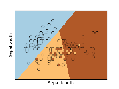
Figure: Logistic regression of iris plant species based two features. (Source: scikit-learn)

Generally, logistic regression divides the space into subspaces corresponding to the input features. From the figure above, we can see that, given a new plant observation where the (length, width) features falls inside the blue region, the model will decide that this plant belongs to the “blue” species.

Turning back to our Sherlock application case, we have selected four features as follows.

Given the four features above, we want train a ML model using logistic regression to tell us whether the corresponding application is “WhatsApp” or “Facebook”. Thus the input is a set of four values and the output is only one (categorical) value. The structure of our model is like as follows.

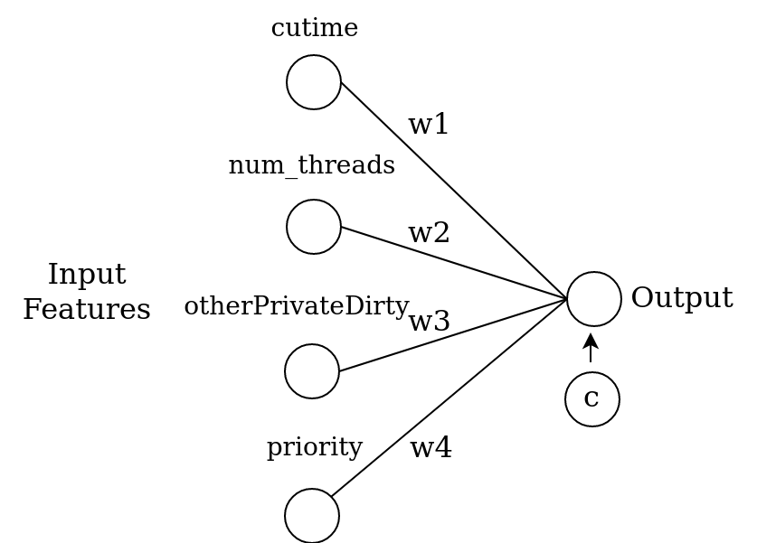
Here, each of the four features will be multiplied by a weight vector (w1, w2, w3 and w4) and summed up (i.e. dot product), and added an extra constant named c:

z = w1 * cutime + w2 * num_threads + w3 * otherPrivateDirty
  + w4 * priority + c

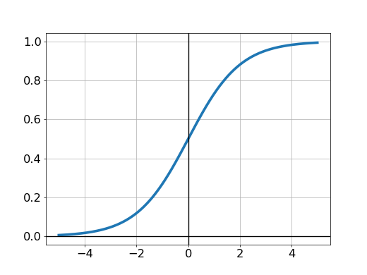
This value is passed to a sigmoid function σ(z) = 1 / (1 + exp(-z)) and output a value which classifies the application: 0 for “WhatsApp”, and 1 for “Facebook”. The training set is used to determine the optimal values of the weights and constant c. The validation set is used to evaluate the performance of the trained model. Here is the plot of the sigmoid function:

The systematic tutorial including the fundamental mathematics for logistic regression can be found in notes from Andrew Ng’s lecture.

Decision Tree

Decision tree is a different approach to machine learning. Instead of using a smooth function, this method employs multiple condition-based branches in order to determine the classification of the input data. Below is an llustration of a decision tree for the Iris dataset:

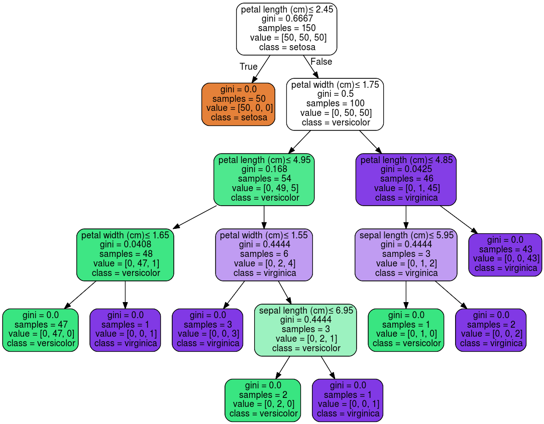
Figure: A 3-feature decision tree for Iris dataset. (Source: scikit-learn)

This decision tree has three features as its input: petal length, petal width, and sepal length. To perform its classification task, we trace the (upside down) tree from the top. At the first branching point, we check whether the petal length is less than or equal to 2.45 cm (topmost white box). If this condition is true, then the plant belongs to the “Iris setosa” species. If not, the model will check whether the petal width is no more than 1.75 cm (the second white box). The vector with three numbers (such as value=[0,50,50] refers to the number of remaining members for each of the three classes. Specifically, at the top, we can see that there are 50 samples for each class. The gini impurity is the probability that a sample, randomly chosen from the current set, would be wrongly classified. The goal of parameter optimization for a decision tree is to minimize this error at all the final points by determining the best branching points and what condition to test on each branching point. The number of branches and the maximum depth of each branch are two examples of hyperparameters in decision tree. Another choice of hyperparameter would be the stopping criterion: in the example above we use the gini criteria (to minimize it). Another possible criterion is the maximization of “information gain”—therefore this chouce of “gini impurity” or “information gain” is an example of hyperparameter that is not a number!

Initial Explorition to Decision Tree

1. Try to explain each box in the trained decision tree.
2. Think about which number should the training determine.
3. Think about which metric can we use to measure the goodness of the model.

Solution

The threshould in each box should be determined by training.

The gini can be utilized to measure the goodness of the model. The smaller, The better.

Note: A systematic introduction to decision tree can be referred here.

Logistic Regression or Decision Tree?

Some simple guidances may help us to choose logistic regression or decision tree under our own scenario.

1. Logistic regression is more suited for classification tasks that are linearly separable in the feature space. While decision tree can better handle nonlinear classification. Thus, if you are certainly sure that the dataset can be linearly separated, try logistic regression first. Otherwise try decision tree first.

2. If the output data type is category, you can try decision tree first, and if the output data type is continuous, try logistic regrassion first.

Decide the First Algorithm to Test in Our Case

1. Which algorthm can be the first best shot for Sherlock application dataset, considering the rule 1 above?
2. Discuss which algorithm can be first considered based on rule 2 above.
3. Can you make a conclusion to choose which algorithm in our case?

For more comparison between logistic regression and decision tree, see here.

Building and Training Model

Now we are ready to to build our model based on our dataset. Recall that we have split the dataset into training set and testing set. The data structure is: train_data, test_data, train_label, test_label.

Discussion of the Split Data

1. What is the dimension of each of four split data?

2. Try to print the size of the above four split data and verify your answer to the first question.

We now use train_data and train_label to build and train our model.

Build and Train Decision Tree Model

We use the DecisionTreeClassifier in scikit-learn to build and train the decision tree model:

from sklearn.tree import DecisionTreeClassifier
model_dtc = DecisionTreeClassifier(criterion='entropy', max_depth=6, min_samples_split=8)
model_dtc.fit(train_data, train_label)

Discussion on the Selection of Classifier Parameters

1. Try to figure out what dose each command do?

2. Try to explain the meaning of selected values by referring here.

Build and Train Logistic Regression Model

We then use the LogisticRegression in scikit-learn to build and train the logistic regression model:

from sklearn.linear_model import LogisticRegression
model_lr = LogisticRegression(solver='lbfgs')
model_lr.fit(train_data,train_label)

Discussion on the Selection of Classifier Parameters

1. Try to figure out what dose each command do?

2. Try to explain the meaning of selected values by referring here.

Test Your Model

After train our models, we want to evaluate them by using the testing set, which includes test_data and test_label. We can also get the statistic of the traied model by using training set.

Write the Evaluation Function

We want use confusion_matrix accuracy_score, precision_score and recall_score to see the model performance. We define the evaluation function as follows.

from sklearn.metrics import accuracy_score, precision_score, recall_score, confusion_matrix
def model_evaluate(model,train_data,test_data,train_label,test_label):
    train_L_pred = model.predict(train_data)
    dev_L_pred = model.predict(test_data)
    print("Evaluation of training set by using model:",type(model).__name__)
    print("accuracy_score:",accuracy_score(train_label, train_L_pred))
    print("No of correct:",accuracy_score(train_label, train_L_pred, normalize=False))
    print("precision_score:",precision_score(train_label, train_L_pred))
    print("recall_score:",recall_score(train_label, train_L_pred))
    print("confusion_matrix:","\n",confusion_matrix(train_label, train_L_pred))
    print("Evaluation of development set")
    print("accuracy_score:",accuracy_score(test_label, dev_L_pred))
    print("confusion_matrix:","\n",confusion_matrix(test_label, dev_L_pred))
    return 

Learning the Performance Metrics

1. Click the link for each performance metric to understand the meaning.
2. Exchange your understanding with others.

Measure the Goodness of Your Models

After we have the evaluation function, we can use it to evaluate our trained model by

# for decision tree classifier
model_evaluate(model_dtc,train_data,test_data,train_label,test_label)

# for logistic regression
model_evaluate(model_lr,train_data,test_data,train_label,test_label)

Compare the Performance of the Two Trained Models

1. Explain the evaluation output of each model.

2. Link with the algorithm guidences introduced before discussion which model may be better for our dataset and think the possible reasons.

Beyond the Selected Features: Principal Component Analysis

Till now, we only use the selected original features to build our models. Actually, we can abstract the features based on the existing features. Specifically, the Principal Component Analysis (PCA) is one of the popular feature abstraction method. Simply speaking, the PCA transform the current features into a newly set of features, which retains most properties of original data. We can do PCA to abstract our selected features by

from sklearn.decomposition import PCA
pca = PCA(n_components=2)
principalComponents = pca.fit_transform(df)
principalDf = pd.DataFrame(data = principalComponents, columns = ['principal component 1', 'principal component 2'])
principalDf.head(10)

Using the New Features

1. Use the newly obtaied features to rebuild, retrain and re evaluate the decision tree and logistic regresion models.
2. Try to change the n_components in the above script and repeat the first step. Discuss the results with different n_components.

Key Points

• Logistic regression and decision tree are two examples of classic machine learning algorithms.

• Learn to fit the model with training set and test the model with model evaluation function.