Introduction to Machine Learning

Overview

Teaching: 0 min
Exercises: 0 min

Questions

• What is exactly machine learning?

• What can be accomplished by computers through machine learning?

• What are the different types of machine learning?

Objectives

• Understanding the essence of machine learning.

• Understanding the concepts of function, data, and learning process.

Machine learning (ML) is a very hot topic today. There are many variations on the definition of “machine learning”.

• Wikipedia definition:

  Machine learning is the scientific study of algorithms and statistical models that computer systems use to progressively improve their performance on a specific task. Machine learning algorithms build a mathematical model of sample data, known as “training data”, in order to make predictions or decisions without being explicitly programmed to perform the task.

• Stanford definition (from Andrew Ng’s famous “Machine Learning” course):

  Machine learning is the science of getting computers to act without being explicitly programmed.

• Emerj collected several definitions of machine learning by well-known parties and came up to the following conclusion:

  Machine Learning is the science of getting computers to learn and act like humans do, and improve their learning over time in autonomous fashion, by feeding them data and information in the form of observations and real-world interactions.

These are all very compact definitions. In this lesson module, we will learn about some practical ML techniques, therefore acquiring an idea about what ML is and what it can accomplish.

Machine Learning—A Practical Definition

• Machine learning builds and combines knowledge from these disciplines:

  • Mathematics
  • Statistics (and statistical analysis)
  • Computing
  • Domain knowledge

  Domain knowledge is very important in order to make meaningful use of machine learning.

• Machine learning is about discovering patterns from data, and about modeling these patterns.

• Machine learning boils down to finding a mathematical model that can best describe the data: from this model, we can make useful predictions and generalizations.

As we shall learn in this module, machine learning encompasses a class of techniques that share similar features and characteristics.

About Machine Learning Model

A model in the world of machine learning is essentially a mathematical function f(X) -> y.

• It expects one or more numbers (vector X) as the input
• It produces one or more numbers (scalar or vector y) as the output

The input data X are often called “features”. actual output data y (sometimes called “labels” in certain type of machine learning).

This implies that all inputs and outputs to a model needs to be converted to numerical values. Images, videos, words, and everything else needs to be turned to numbers.

Discrete-Valued vs Continuous Functions

The y output of the function could be discrete-valued or continuous.

Continuous functions, which output continuous values (i.e. real numbers) are frequently encountered in science, engineering, business, etc., where the underlying process is continuous in nature. Some examples from engineering and science:

• the relationship between RF signal strength and distance and orientation of the emitting device;

• a network link’s performance such as bandwidth or latency as a function of data sizes and number of the network flows;

• in a chemistry experiment: the relationship between chemical reaction rate and reactant’s concentrations, temperature, pressure, etc.

Continuous functions also appear in popular business applications, such as:

• Estimation or prediction of stock price trend

• Estimation of debt default rate

• Estimation of house price based on its features (count of rooms, total living area of the house, etc.)

In cybersecurity, an example would be modeling a cyberthreat risk given the various factors (such as the number of servers, age of servers, number of published services on the network, etc.)

Discrete-valued functions, which output discrete values, are frequently found in cybersecurity applications—perhaps even more so than continuous function. In most cases, the choice of the values are finite; these functions are well suited for classification tasks. Some examples drawn from cybersecurity are:

• classification of network events as benign or malicious;

• malicious application detection;

• spam detection;

• determination of the type of network flows (whether they are multimedia stream, chat, web, file sharing, etc.).

All of these tasks use functions that return a finite possibilities of discrete values. For example, in spam classification, y=0 means a legitimate email, whereas y=1 marks a spam.

Beyond cybersecurity, functions of this nature are widely used in image classification (cat, dog, car, truck, bus, …), face object detection in image or video, text sentiment analysis. In medicine, example applications include: identification of cancerous cell mass from radiology images, computer-aided diagnosis of disease. In financial world, classification is frequently used in detection of fraudulent transactions.

These two classes of functions will have different machine learning algorithms for each of them, as detailed below.

Learning from Data

The models used in machine learning have (many) parameters, which need to be adjusted to make the models perform prescribed tasks. This overall process of adjusting the model parameters is called training (although as we will see shortly, training involves additional steps to ensure that the resulting models are robust). All machine learning models require data to train them. The more data available to train the model, the more accurate the model captures the pattern of the data.

Types of Machine Learning

Here is a common taxonomy of machine learning techniques:

• Supervised learning

  • Regression

  • Classification

• Unsupervised learning

  • Dimensionality Reduction

  • Clustering

• Semi-supervised learning

• Reinforcement learning

Supervised learning

In supervised learning, the input data X (“features”) come with the actual output data y. The parameters in the model are then adjusted during the training process so that the model would predict the output as accurately as possible.

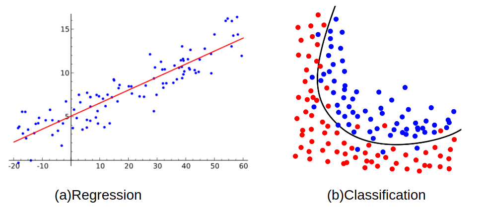
• Regression models are used when the output values are expected to be continuous (i.e. it is an arbitrary real number).

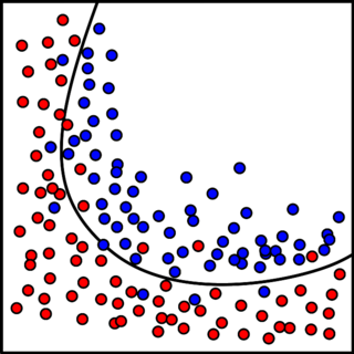
• Classification models are used when y values are discrete-valued and have only finite number of possible values (this kind of y is often called “label”).

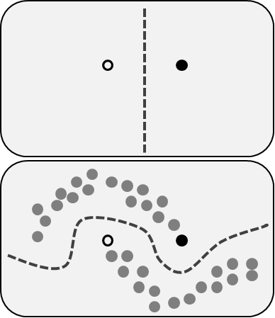
Unsupervised learning

In unsupervised learning, only the input data X are provided. The goal is for an algorithm to recognize the underlying structure in the data.

• One example is dimensionality reduction, aiming at finding the (most) relevant features without losing structural information.

• Another example isclustering algorithm, which is useful to find clusters with similar features.

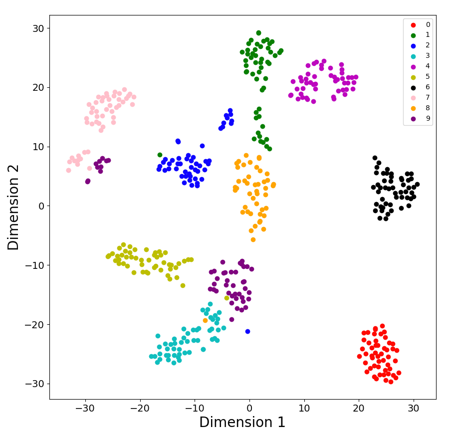
Figure: An example of dimensionality reduction and clustering using Digits dataset — digits in 8×8 = 64 dimensions)

Semi-Supervised learning

Semi-supervised learning falls between unsupervised learning (without any labeled training data) and supervised learning (with completely labeled training data). The input includes both labeled and unlabeled data.

Reinforcement learning

Reinforcement learning differs from supervised learning in not needing labelled input/output pairs be presented, and in not needing sub-optimal actions to be explicitly corrected. Instead the focus is on finding a balance between exploration of current knowledge and exploitation of uncharted territory. It can be applied in various problems, including robot control, cherckers, Go(AlphaGo), video game AI.

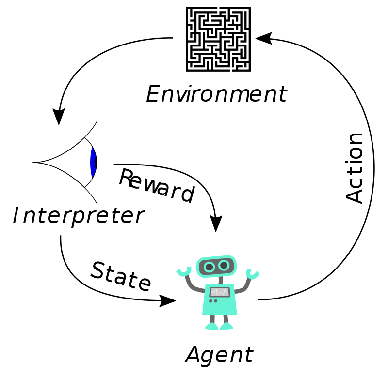
The typical framing of a Reinforcement Learning(RL) scenario like a Markov decision process: an agent takes actions in an environment, which is interpreted into a reward, and a representation of the state fed back into the agent.

Classical Machine Learning Algorithms

In this lesson module, we are focusing on classic ML algorithms—in particular, logistic regression and decision tree. We refer to these as “classic” ML algorithm because they have been around and used much longer than the more recent deep learning (DL) algorithms. The DL algorithms, based on neural networks, have proved to have extremely predictive power and versatile in areas such as image analysis, speech recognition, language translation. While DL algorithms have virtually limitless accuracy (given enough sample to train the networks), they are computationally very expensive to train. DL algorithms are also difficult (if not impossible) to interpret; that is, while DL provides the answer to the “what” question, it is not easy to understand the “why”. Classic ML algorithms are derived from “reason”-able models—those that are understandable to humans. The proper use of classic ML requires more understanding of the data and its features. Many classic ML algorithms do not require huge computational power and they can work well even when the amount of data is not very large.

Basic Steps in Machine Learning

Main stages of machine learning:

1. Train the model—i.e., adjust the model parameters so that f(X) would fit the expected y as best as possible;

2. Validate the model (in terms of accuracy and performance);

3. Adjust the model by tuning its “hyperparameters” (see below);

4. Repeat stages 1–3 until satisfactory model is obtained;

5. (optional) Final test on the model’s accuracy and performance;

6. Use the model for prediction—the deployment stage.

Clearly, machine learning is an iterative process, where stages 1-3 are iterated (and it can be many times before a sastisfactory model can be obtained).

For machine learning, data are typically split into three sets:

1. Training set, used to train the model’s parameters in step 1.

2. Validation set (sometimes also called development or simply dev set), used to perform the validation in step 2.

3. Test set, used to judge the final accuracy of the model in step 4.

In stages 2 and 5, the reserved sets of the data are used to provide an unbiased measure of the performance of the model that was trained/adjusted in previous step. We will describe these three sets and the common practice in a latter episode.

The following “graphics” illustrates the lifecycle of machine learning and the three sets of data:

* MACHINE LEARNING LIFECYCLE *
|
|    (1)           (2)           accuracy                (3)
|  Training --> Validation --> good enough?  (YES) --> Testing --> Deployment
|     ^                           (NO)                  final
|     |          adjust            |                   accuracy
|     +----- hyperparameters <-----+
|
|
|  Datasets used:
|    (1) Training set
|    (2) Validation set
|    (3) Test set
|
*

An important advice regarding the data partitioning:

NEVER EVER MIX data that are used for the training, validation, and test sets!

Parameters and Hyperparameters

What makes machine learning powerful is that the model contains parameters that can be systematically improved accoding to a prescribed algorithm. Parameter adjustment is automated, i.e. not requiring human labor in the process. The adjustment of model parameters takes place in the training stage (step 1) through an iterative optimization algorithm.

In addition, machine learning models frequently also have adjustable constants called hyperparameters, which affect the final accuracy of the model. Hyperparameters do not get optimized in the training stage. In fact, at this point in time, there is no way for hyperparameters to be “optimized” in the way parameters are optimized:

• There is no systematic formula on how to update hyperparameters based on the change in the model’s validated accuracy. (At least, there is not yet. This is currently an active research area. For example, today some people are using yet another “machine learning” on top of the original machine learning in order to automatically optimize the hyperparameters in a smart way.)

• Some hyperparameters are not even numeric! The examples later in the Drones dataset will make this clear.

• We do not know a priori what is the “best possible” performance of a machine learning model for a given problem. Let’s say, we have a dataset of network events with all the carefully selected features, and we are tasked to build a model that can predict which events are malicious. There is no formula to estimate that the accuracy of the “decision tree” algorithm on this specific problem. (It would be very nice if such a formula exists, that claims that decision tree would yield at least 90% accuracy.)

Most of the time, machine learning is a “loop-within-loop” iterative process, where the adjustment of model parameters (training stage) is carried out using an iterative optimization algorithm, and the iterative tuning of hyperparameters becomes the “outer loop” which requires human judgment and intervention. For this reason, machine learning tends to be computationally intensive, thus often needs HPC or a lot of computers to shorten the time to build a good model.

Assessing Quality in Machine Learning

Although many steps in the machine learning lifecycle can be automated, we (humans) eventually must exercise our sense of judgment on the quality and reliability of the model. All in all, machine learning needs to be used with care; we should not blindly treat and trust machine learning as a blackbox.

Bias and Variance—Issues with Underfitting and Overfitting

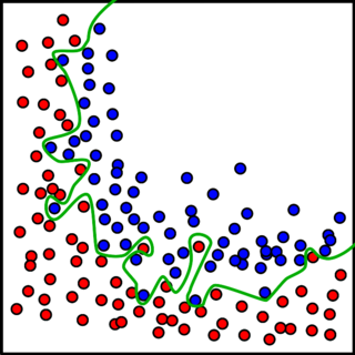
Overfitting (high variance):

Underfitting (high bias):

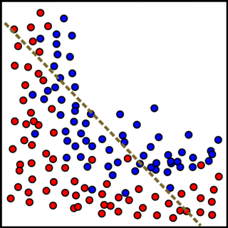
“Just right” fitting:

Accuracy, Precision, Recall, Confusion Matrix

Precision and recall:

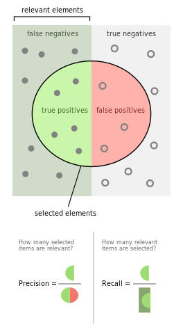
Intuitively speaking:

• precision is the ability of the classifier not to label as positive a sample that is negative (i.e. to avoid false positives);

• recall is the ability of the classifier to find all the positive samples.

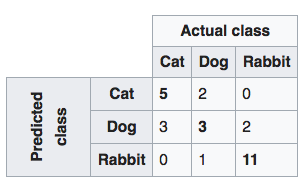
Confusion matrix, or table of confusion:

Key Points

• Machine learning methods are divided into two classes: supervised and unspervised.

• Supervised ML methods train models based on given data with labels/outcomes/objectives.

• Unsupervised ML methods aims at finding structure/pattern without labeling the data.