Analytics of Sherlock Data with Pandas

Overview

Teaching: 30 min
Exercises: 20 min

Questions

What are the basic data manipulation operations (building blocks) in pandas?

What insights can we obtain by common combinations of these building blocks?

Objectives

Become familiar with data analysis in pandas

Learning building blocks of data manipulation

Introduction

In this episode, we will build upon the foundation of DataFrame and Series introduced in the previous episode to perform various analyses and extract insights from the Sherlock data. These will be carried out by building pipelines out of several basic building blocks in data manipulation:

Column selection and transformation
Filtering (i.e., conditional row selection)
Grouping
Aggregation
Merging tables
Sorting

Those who know SQL (Structured Query Language) would realize that these are also the basic operations in SQL.

We will learn to use these building blocks to answer statistical questions beyond the most basic ones like:

“What’s the average memory usage?”
“What’s the maximum number of threads?”
“What is the median value of lru?”

We can ask more specific question, such as:

“What’s the average memory usage for each application?”
“What’s the memory usage across all applications for a range of time instances?”
“Which application consumes the most memory on May 16?”
“Which application consumes the most CPU cycles?”
“What is the memory usage pattern (over time) for different kinds of messaging applications?”

About `Applications.csv` Table

Reading sherlock_mystery.csv

For the exercises in this episode, please make sure you already loaded the sherlock_mystery.csv data file. Name the variable df_mystery.
df_mystery = pandas.read_csv('sherlock/sherlock_mystery.csv')

Peeking into the dataset

Always take a look at your dataset first before doing anything else! Hint: The describe(), shape, dtypes methods/attributes are particularly useful.

Try to answer the following questions:

How many rows and columns are in this dataset?

How do the numbers look like?

How does the statistical information look like?

What does the feature look like? (i.e. the data types)
Solution
print(df.shape)
print(df.head())
print(df.describe())
print(df.dtypes)

First few rows of df_mystery

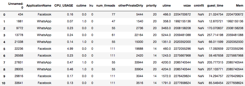
Figure: First few rows of df_mystery. (The output is truncated horizontally. There are more columns to the right of the table shown above.)

Features

The sherlock_mystery.csv contains 14 columns (features) and 200 rows (records). The column names describe the information stored in this dataset, as listed below:

Unnamed: 0 [int]: The original position of the record in the Application.csv file.
CPU_USAGE [float]: The percent of CPU utilization (100% = completely busy CPU).
cutime [int]: Amount of CPU “user time” spent the spawned (child) processes, measured in clock ticks.
lru [int]: “An additional ordering within a particular Android importance category, providing finer-grained information about the relative utility of processes within a category.” (SherLock’s documentation) This is an Android OS parameter. LRU stands for “Least Recently Used”. Here, lru is a parameter in the application memory management.
num_threads [int]: Number of threads in this process.
otherPrivateDirty [int]: The private dirty pages used by everything else other than Dalvik heap and native heap.
priority [int]: The process’s priority in terms of CPU scheduling policy.
utime [int]: Amount of the CPU “user time”, measured in clock ticks.
vsize [int]: The size of the virtual memory, in bytes.
cminflt [int]: The number of minor faults that the process’s child processes.
guest_time [int]: Amount of the time running the “virtual CPU”, measured in clock ticks.
Mem [int]: Size of memory, in bytes.
queue [int]: The waiting order (priority).

As you can see, these parameters provide very intimate, machine-level information about the apps running on the smartphone. One column is not described here, which is the ApplicationName. This is the name of the application whose features are measured and stored together with the other 13 columns.

Wanting More Information?

Data in Applications.csv were collected by the SherLock agent from the participant’s smartphones. The SherLock agent made frequent, periodic probes (“polls”) of system variables at a high resolution (about 5 seconds apart between adjacent probes), leading to a detailed view of the history of apps running on these phones.

The information about the columns above is abridged. For more precise definition, please refer to Linux man page for proc(5), under the description for /proc/[pid]/stat.

For this lesson, we select only a few columns from the full Applications.csv table, which has a total of 57 features. Detailed description of all the tables available in the entire Sherlock dataset is available online in PDF format.

Column Selection

In analytics, we often need only a few columns from the full table. We have covered column selection in the previous episode, using the [] operator. Several examples:

# Select only memory statistics & the application name
df_memstats = df_mystery[['ApplicationName',
                          'vsize', 'Mem', 'otherPrivateDirty']]

# Select only processor statistics & the application name
df_cpustats = df_mystery[['ApplicationName',
                          'CPU_USAGE', 'utime', 'cutime', 'guest_time']]

Statistics of Selected Columns

Examine the contents of df_memstats and df_cpustats from the example above. Also print the descriptive statistics of the data. Wouldn’t these look a lot better—not much clutter compared to printing the statistics for all the columns on the master table?

Solution

print(df_memstats.describe())

              vsize           Mem  otherPrivateDirty
count  2.000000e+02  2.000000e+02          200.00000
mean   2.175793e+09  2.175793e+09        20426.28000
std    1.417478e+08  1.417478e+08        23323.22431
min    1.983623e+09  1.983623e+09           32.00000
25%    2.095809e+09  2.095809e+09         2826.00000
50%    2.107628e+09  2.107628e+09        13552.00000
75%    2.252854e+09  2.252854e+09        29993.00000
max    2.633560e+09  2.633560e+09       114972.00000

print(df_cpustats.describe())

        CPU_USAGE         utime      cutime   guest_time
count  200.000000    200.000000  200.000000   200.000000
mean     0.224750   4224.705000    0.420000   207.781320
std      0.417532   5493.086456    0.926223   274.703022
min      0.000000     23.000000    0.000000    -4.436543
25%      0.080000    559.750000    0.000000    24.585457
50%      0.160000   2238.500000    0.000000   109.155168
75%      0.270000   6457.000000    0.000000   318.810321
max      4.990000  34615.000000    4.000000  1725.901364

Much easier to look for the quantities of interest than the previous one, right?

Removing Columns

Whereas the [] operator selects which column(s) to include, we can use the drop method to discard certain columns (or rows) from the DataFrame. In our df_mystery, the column named Unnamed: 0 carries information which is irrelevant to us—it simply records the original row label in the original dataset. Therefore we can get rid of it by:

df_mystery2 = df_mystery.drop('Unnamed: 0', axis=1)

(The axis=1 is needed because by default the drop method will eliminate rows whose label is given.) We can also drop multiple columns:

# Drops useless feature and the ApplicationName (which is not a feature):
df_features_only = df_mystery.drop(['Unnamed: 0', 'ApplicationName'], axis=1)

By default, the drop method returns a new DataFrame object, leaving the original DataFrame unchanged. We do not have to always specify a new variable. We can do the following:

df_mystery = df_mystery.drop('Unnamed: 0', axis=1)

Or better yet, in this case we should perform an “in-place” operation, which will not produce a new DataFrame object:

df_mystery.drop('Unnamed: 0', axis=1, inplace=True)

The drop method used in this way will return nothing.

Column Operations

pandas made it convenient to operate on Series and columns of DataFrame. For example, we can perform arithmetic operations on one or more columns. We will show these capabilities through examples below.

Arithmetic Operations

Case 1: Converting units from bytes to gigabytes—arithmetic between a column and a scalar value

vsize_gb = df_mystery['vsize'] * 1e-9
print("Original data:")
print(df_mystery['vsize'].head())
print("Same data in units of GB:")
print(vsize_gb.head())

Original data:
  2204700672
  1992155136
  2008158208
  2059481088
  2020352000
Name: vsize, dtype: int64
Same data in units of GB:
  2.204701
  1.992155
  2.008158
  2.059481
  2.020352
Name: vsize, dtype: float64

pandas will perform element-wise arithmetic and return a new Series object with the same index as the input data (the vsize column). (Since the second operand is a scalar (1e-9), every element in the vsize column will be multiplied by this number.) It is very common to store the new Series in a new column in the same (or different) DataFrame:

df_mystery['vsize_gb'] = df_mystery['vsize'] * 1e-9

Please verify that now df_mystery has one additional column.

NOTE: We can also update the existing column to contain the transformed values by reusing the same column name in the assignment, e.g.

df_mystery['vsize'] = df_mystery['vsize'] * 1e-9

Case 2: Subtracting guest_time from utime—arithmetic involving multiple columns

df_mystery['utime_self'] = df_mystery['utime'] - df_mystery['guest_time']
print(df_mystery[['utime', 'guest_time', 'utime_self']].head())

    utime  guest_time   utime_self
 466.0   21.024754   444.975246
 358.0   12.870721   345.129279
3463.0  170.070837  3292.929163
5244.0  257.714198  4986.285802
1351.0   66.011599  1284.988401

Vectorized Operations for High Performance

(Advanced Notes) The two examples above serve as an illustration of vectorized operations in Python`. They operate on Series objects as if these objects were ordinary Python variables, and yield a new Series. Since Series is analogous to an array, or a vector, the operation will act on many elements at once. Behind the scenes, pandas will perform this computation in highly optimized functions written in C or C++, therefore achieving high performance.

It is important to note that the elements from the different input Series are matched by the row labels (i.e. by the index). Consider the last operation:
df_mystery['utime_self'] = df_mystery['utime'] - df_mystery['guest_time']
Behind the scenes, this actually involves a loop:
# a C-like analog of the expression above:
for i in df_mystery.index:
    df_mystery.loc[i, 'utime_self'] = df_mystery.loc[i, 'utime'] \
                                    - df_mystery.loc[i, 'guest_time']
Those new to pandas with programming experience in compiled languages like C, C++, Fortran might be tempted to program in this way. But employing this approach in Python would result in terrible performance, because Python is an interpreted language, therefore it has a high overhead for each statement being executed. In general, we need to think in the pandas way: Are there pandas constructs, operators, or functions that would achieve our goal without explicitly looping over the data elements? A blog article titled “Fast, Flexible, Easy and Intuitive: How to Speed Up Your Pandas Projects” chronicles a real-life experience of speeding up data processing by using proper pandas constructs.

In cases where we require hand-crafted functions or operations beyond what pandas standard library provides, we recommend interested readers to start with “Enhancing Performance” chapter in pandas user’s guide. This is an advanced topic, beyond the scope of this lesson, therefore we will not discuss it further.

String Operations

A Series object has a str attribute, which contains an extensive collection of string functions. Consider an example case where a column contains information that was entered by humans, e.g. via a web form. This data tend to be messy with different character cases: Facebook, facebook, FACEBOOK and even worse, faceBOOK. To make these values more consistent, we need to convert all letters to just one kind of case. We can do one of the following:

df_mystery['APPNAME'] = df_mystery['ApplicationName'].str.upper()
# -- or --
df_mystery['appname'] = df_mystery['ApplicationName'].str.lower()

The vectorized string functions such as upper and lower methods above typically have names and functionalities that are identical to the methods of Python string (e.g. str.upper, str.lower, etc.). Some vectorized functions have the their names and meanings borrowed from the re (regular expression) module. We are not going to discuss the string capabilities further, because we do not need to work with strings in the Sherlock application dataset.

Those that need to work with text data can learn more from pandas User’s Guide, most notably:

Working with Text Data: https://pandas.pydata.org/pandas-docs/stable/user_guide/text.html
Summary of String Methods in pandas: https://pandas.pydata.org/pandas-docs/stable/user_guide/text.html#method-summary

Applying Custom Transformations

We can apply custom transformation for each value in a DataFrame or Series by defining a Python function. Let’s redo the “conversion to gigabytes” in this way:

def to_giga(val):
    return val * 1e-9

df_mystery['vsize_gb2'] = df_mystery['vsize'].apply(to_giga)

An example of a more complex function:

def non_negative(val):
    if val > 0:
        return val
    else:
        return 0

df_mystery['guest_time_fix'] = df_mystery['guest_time'].apply(non_negative)

This function is supposed to fix all negative numbers to zero, because we do not expect guest_time to be negative. Please check the values of guest_time_fix are fixed (no more negative values).

Note: DataFrame.apply method also exists, but it performs the operation on column-by-column basis (or row-by-row basis if axis=1 argument is given), and return a Series object. To perform element-by-element application of the function, use DataFrame.applymap method instead (which still returns a DataFrame object).

Computing Range of Column Values

A student named Lee wants to compute the range of the values for each column. He wrote the following code:
def value_range(col):
    return max(col) - min(col)

print(df_mystery.apply(value_range))
He ran this code, but it failed with an error. He scratched his head—What’s wrong with my code? He said. Can you troubleshoot his and help him fix his code?
Hint

Here is the error message (at the end of a long stack dump):
[...]
<ipython-input-43-e566e18dabe2> in value_range(col)
      1 def value_range(col):
----> 2     return max(col) - min(col)
      3
      4 print(df_mystery.drop('ApplicationName',axis=1).apply(value_range))

TypeError: ("unsupported operand type(s) for -: 'str' and 'str'", 'occurred at index ApplicationName')
The error was encountered because the ApplicationName column contains non-numeric data.
Extra Challenge!

Actually, the problem above is a perfect example on how we can apply pandas built-in capabilities to compute the range. The is a better and faster way to get the result without using the apply() method.

Hints:

One of the functions we covered in the previous episode did return the minimum and maximum values for each column: Which one is that? We can use the result of that method to compute the range!

A correct implementation can be had with only two lines of code! How can we take advantage of that function?

Filtering

Boolean Expressions

Now we come to a special type of expressions which return only True or False values. This type of expressions is useful for filtering data, which we will cover next.

Let’s consider our Sherlock data again. Sir Hitchcock, the user of the phone which produced our data, complained that his phone was not responsive at certain times. He suspected that either WhatsApp or Facebook was the culprit. So, as a computer detective with Applications.csv at our disposal, let’s hunt for some clue. Where should we start? We may suspect that one of these processes may crank up the CPU for a long time. The Sherlock data contains CPU_USAGE column which measures the instantaneous usage of the CPU in units of percent (100 means that the CPU is fully busy).

We can compare a column (i.e. a Series) with a value, e.g.

df_mystery['CPU_USAGE'] > 50

This returns a Series of Boolean values: True where the corresponding CPU_USAGE value is greater than 50, False otherwise.

First Investigation: Examining CPU Usage

The following expression will return True on rows where CPU_USAGE field is greater than 50%:
print(df_mystery['CPU_USAGE'] > 50)
What are the values you see? Any row containing True? If not, why? Can you explain it?

Hint

Consider the statistics given by the describe method earlier.

Let’s drop the threshold to 20%, 10%, 5%, and 2%. Where did you start seeing True values? Can you count how many records match the condition above?
Solution

We find some nonzero value at 2% threshold. We can use the sum method of the resulting expression to count how many records satisfy this condition.
print((df_mystery['CPU_USAGE'] > 2).sum())
2
When summing over values, a True value is equivalent to a numeric 1, and False is equivalent to zero. The extra parentheses surrounding the Boolean expression are required so that the > comparison operator is evaluated first before the sum method is called.

The effort to find high CPU_USAGE value turns out to be futile. Even finding a non-negligible value turns out to be like finding needles in a haystack!

Filtering Rows

What happens if we combine the comparison expresion above and the DataFrame[] operator? We have a way to filter rows based on a given criterion. Let’s apply this to the investigation above:

print(df_mystery[df_mystery['CPU_USAGE'] > 2])

    Unnamed: 0 ApplicationName  CPU_USAGE  cutime  lru  num_threads  \
5        22236        Facebook       4.99     0.0    0          111
99      386844        Facebook       2.78     0.0    0           79

    otherPrivateDirty  priority  utime       vsize  cminflt  guest_time  \
5               19688        14  460.0  2272055296      NaN   17.092659
99              31292        20  793.0  2202218496      0.0   35.518860

           Mem       queue  utime_self  vsize_gb2
5   2272055296  121.428571  442.907341   2.272055
99  2202218496  100.000000  757.481140   2.202218

Using the right tools in pandas, it is rather easy to locate difficult-to-find records!

Boolean expressions can be combined using the AND (&) or OR (|) bitwise operators. The NOT operator is a (~) prefix against a Boolean expression. However, the conditions must be enclosed with () because of Python’s priority of operators. Some examples:

# AND operator
(df_mystery['ApplicationName'] == 'Facebook') \
    & (df_mystery['CPU_USAGE'] > 0.5)

# OR operator
(df_mystery['ApplicationName'] == 'Facebook') \
    | (df_mystery['CPU_USAGE'] > 0.5)

# NOT operator
~(df_mystery['CPU_USAGE'] > 0.5)

Note: The standard Python logical operator (and and or) cannot work for vectorized logical expression like the above.

Investigation Continued

Examine the df_mystery filtered by the composite conditions above. How many records did we find for each case?

Solution

The expression with the AND operator returns only 7 rows (row labels: 5, 99, 144, 145, 189, 191, 192).

The expression with the OR operator returns 126 rows (row labels: 0, 5, 6, 9, 10, 11, …).

The expression with the NOT operator returns 188 rows (row labels: 0, 1, 2, 3, 4, 6, 7, 8, …).

How do we count the number of rows without making a DataFrame? For example: how many rows of non-WhatsApp data that have CPU_USAGE values greater than 0.5?

Hint

Use the composite Boolean expression and the sum method.

Summary of Common Boolean Expressions

The following table lists common logical expression patterns that are frequently used inside the filter() argument. Each operation is evaluated elementwise against the data in COLUMN; the result is stored in a new Column that has logical values (only True or False).

Description	Commonly Used Syntax	Example
Value comparison (numerical or lexical)	`COLUMN == EXPR`	`df['num_threads'] == 80`
	`COLUMN != EXPR`	`df['num_threads'] != 80`
	`COLUMN > EXPR`	`df['num_threads'] > 80`
	`COLUMN >= EXPR`	`df['num_threads'] >= 80`
	`COLUMN < EXPR`	`df['num_threads'] < 80`
	`COLUMN <= EXPR`	`df['num_threads'] <= 80`
String match (exact comparison)	`COLUMN == 'SOME_STRING'`	`df['App'] == 'WhatsApp'`
String mismatch (exact comparison)	`COLUMN != 'SOME_STRING'`	`df['App'] != 'WhatsApp'`
Exact match at beginning of the string value	`COLUMN.str.startswith('SOME_STRING')`	`df['App'].str.startswith('Google')`
Exact match at end of the string value	`COLUMN.str.endswith('SOME_STRING')`	`df['App'].str.endswith('App')`
Exact match located anywhere in the string value	`COLUMN.str.find('SOME_STRING') >= 0`	`df['App'].str.find('soft') >= 0`
Regular expression match on the string value	`COLUMN.str.match('REGEXP')`	`df['App'].str.match('.*App')`
Value is defined	`COLUMN.notna()`	`df['cminflt'].notna()`
Value is undefined (i.e. missing)	`COLUMN.isna()`	`df['cminflt'].isna()`
Value is within specified choices of value	`COLUMN.isin(LIST_VALUE)`	`df['App'].isin(['Google Maps', 'Waze'])`

Sorting

Data sorting is a process that orders the data according to certain rules (usually numerical or alphabetical order) to make it easier to understand, analyze or visualize the data. For example, we may want to find applications that hog computer resources by sorting them by the CPU usage, or memory usage, or network traffic volume.

Limit the columns

For this section, let’s limit the columns of the DataFrame object:
# Limit the columns and make copy
df = df_mystery[['ApplicationName', 'CPU_USAGE', 'num_threads', 'vsize', 'utime', 'cutime']].copy()
We will use this disposable df for experimentation.

Let us find the records in df_mystery that indicate the following:

High CPU usage
High memory usage
High number of threads

# Limit the columns
df = df_mystery[['ApplicationName', 'CPU_USAGE', 'num_threads', 'vsize', 'utime', 'cutime']]
df_CPU_hog = df.sort_values(by='CPU_USAGE', ascending=False)
print(df_CPU_hog.head(20))

    ApplicationName  CPU_USAGE  num_threads       vsize    utime  cutime
        Facebook       4.99          111  2272055296    460.0     0.0
       Facebook       2.78           79  2202218496    793.0     0.0
      Facebook       0.92           18  2123202560    684.0     0.0
      WhatsApp       0.87           49  1986613248    336.0     4.0
      WhatsApp       0.61           65  2107408384   3112.0     0.0
      Facebook       0.60          178  2482688000   7944.0     0.0
      WhatsApp       0.58           61  2100404224   2001.0     3.0
      Facebook       0.58          152  2490462208   8606.0     0.0
      Facebook       0.56          152  2490544128   8613.0     0.0
      WhatsApp       0.55           63  2068492288   3274.0     0.0
      WhatsApp       0.53           47  1984712704   2148.0     3.0
      Facebook       0.52          178  2482524160   8552.0     0.0
      WhatsApp       0.49           53  1997946880    690.0     3.0
      WhatsApp       0.47           46  1983623168   2170.0     3.0
        WhatsApp       0.47           55  2085740544   4200.0     1.0
      WhatsApp       0.46           61  2107846656   2126.0     3.0
       WhatsApp       0.46           51  1996378112   2150.0     2.0
        WhatsApp       0.46           55  2085740544   4204.0     1.0
      WhatsApp       0.45           93  2299740160  26698.0     0.0
      WhatsApp       0.45           57  2065424384   1715.0     4.0

In this example, the CPU_USAGE values are used as the sorting key to determine the order of the records.

Sort Capabilities

DataFrame.sort_values by default sorts the records based on the specified columns. DataFrame.sort_index by default sorts the records based on the index. The sort functions in pandas have a large number of capabilities; we feature some of them that are frequently utilized:

The by argument can be a single column name (like the example above) or a list of column names.

By default these methods sort in ascending order (numerical/lexicographical). The ascending argument can be set to False to reverse the sort order. More precise control can be achieved by a list of boolean values.

The inplace=True argument can be specified to sort the data in-place, without creating another DataFrame object.

By default, the sort methods perform the sorting of rows (i.e. axis=0). The axis=1 argument can be specified to make sort_values and sort_index sort the columns based on the values in the specified rows(s).

Practice

Sort the df DataFrame by the values of column CPU_USAGE and utime.
Solution
print(df.sort_values(by=['CPU_USAGE','utime'],ascending=False))

Aggregation (Data Reduction)

Many valuable insights from data analytics do not come from identifying an individual observation (for which sorting and filtering can help), but by aggregating many observations. Aggregation is a process of reducing a set of values to a single quantity (or a handful quantities). The quantities below are obtained from aggregation process:

the top 10 most used application;
the average memory usage over a period of time;
the fluctuation of the memory usage over a period of time;
the total CPU utilization over a period of time.

Many of these are statistical quantities, such as the average, median, standard deviation, sum, minimum, maximum, etc.

pandas provides common aggregation functions as methods that can be applied to both the DataFrame and Series objects:

df.max() — returns the maximum value
df.min() — returns the minimum value
df.mean() — returns the mean (average) of the values
df.sum() — returns the sum of the values
df.mode() — returns the most frequently occuring values (there can be multiple values of such).
df.median() — returns the median of the values

These are some commonly used functions. Yes, we can already obtain them using the df.describe() function; but in general, we only care about one or a few quantities. Therefore in analytics we frequently use these individual functions.

Aggregation Exercises

Can you try the commands below and make sense of the output?
df.max()
df['lru'].mean()
df['ApplicationName'].mode()
df['cutime'].median()
df['cutime'].sum()
df.max(axis=1, numeric_only=True)
Explanation

For a dataframe, df.max() returns the maximum value of each column instead of the maximum value of the entire dataframe.

For string columns, max() will return the highest value according to the lexicographical order.

The axis is used to control the direction of the aggregation: (0 = row-wise, which is the default; 1 = column-wise).

Grouping

In analytics we can also ask detailed questions that involve grouping in addition to aggregation, such as:

What is the maximum memory usage for each application?
What is the average number of threads for each application?
What is the total CPU usage for each application?

The questions above require separating the rows according to the corresponding application names. Here, the application name serves as the grouping key. Then for each group, we can apply analysis or aggregation. This operation is commonly termed “group by”, a process that involves one or more of the following steps:

Splitting the data into groups based on the defined criteria;
Applying a function to each group independently;
Combining the results into a data structure.

pandas provides a convenient way to perform such an operation using the groupby method.

Here are several examples:

Maximum memory usage for each application

print(df.groupby('ApplicationName')['vsize'].max())

ApplicationName
Facebook    2633560064
WhatsApp    2299740160
Name: vsize, dtype: int64

Total CPU cycles spent by each application

print(df.groupby('ApplicationName')['utime'].sum())

ApplicationName
Facebook    397486.0
WhatsApp    447455.0
Name: utime, dtype: float64

In the examples above we want to aggregate just one quantity; so the output of the aggregation is a Series object.

Descriptive statistics for CPU, threads, and memory, calculated per application:

# Preselect columns before doing groupby:
df2 = df[['ApplicationName', 'CPU_USAGE', 'num_threads', 'vsize']]

print(df2.groupby('ApplicationName').describe().T)

ApplicationName        Facebook      WhatsApp
CPU_USAGE   count  1.210000e+02  7.900000e+01
            mean   1.933058e-01  2.729114e-01
            std    5.227195e-01  1.432691e-01
            min    0.000000e+00  7.000000e-02
            25%    0.000000e+00  1.650000e-01
            50%    1.100000e-01  2.400000e-01
            75%    1.700000e-01  3.300000e-01
            max    4.990000e+00  8.700000e-01
num_threads count  1.210000e+02  7.900000e+01
            mean   7.908264e+01  5.954430e+01
            std    5.711941e+01  7.182239e+00
            min    1.100000e+01  4.600000e+01
            25%    1.200000e+01  5.600000e+01
            50%    8.400000e+01  6.000000e+01
            75%    1.330000e+02  6.300000e+01
            max    1.900000e+02  9.300000e+01
vsize       count  1.210000e+02  7.900000e+01
            mean   2.241524e+09  2.075118e+09
            std    1.428934e+08  5.367138e+07
            min    2.093793e+09  1.983623e+09
            25%    2.098053e+09  2.043097e+09
            50%    2.218504e+09  2.085741e+09
            75%    2.349343e+09  2.104979e+09
            max    2.633560e+09  2.299740e+09

Discussion

Discuss some interesting observations from the per-application statistics above.

Solution

These are just some possible answer. There are many more awaiting your exploration.

We have more Facebook records than WhatsApp.

Facebook uses more threads than WhatsApp: Facebook’s maximum number of threads is more than double of WhatApp’s.

In terms of vsize, both applications are about the same in memory usage statistics.

The last .T operator transposes the output dataframe to make it more readable.

Combining Multiple Datasets

Real-world big data analytics will involve integrating datasets in various forms and from various sources. The real Sherlock experiment data is an example of this. The Applications data was collected from the Linux procfs interface. There are also many other tables recording the user’s geolocation (from GPS reading), gravitometer data and other sensors, Wi-Fi environment, battery status, installed apps status, etc. These all will have to be combined and/or correlated to obtain the “big picture” of the security posture of the phone at any time.

For table-like datasets, there are two primary ways to combine datasets:

Adding more measurements of the same kind, which means to add rows into our existing table. This is done by concatenating the two or more tables together.
Adding different but related features from other source(s), which technically inserts additional columns into our existing table. This is done by merging or joining two tables.

Concatenating Datasets

The current dataset (df_mystery) is miniscule to obtain any meaningful statistics. It also contains only data from two application. Supposed that a new set of measurements just arrived in the server; now we want to combine the two datasets into one (larger) dataset.

However, we cannot just combine the two because they have different columns. For the sake of illustration, let us simply perform column selection so that only common columns are obtained, then we can combine the datasets.

# Load all datasets again

cols = ['ApplicationName',
        'CPU_USAGE', 'utime', 'cutime',
        'vsize',
        'num_threads']

# We already preselect columns that we read:
df_set1 = pandas.read_csv("sherlock/sherlock_mystery.csv", usecols=cols)
df_set2 = pandas.read_csv("sherlock/sherlock_head2k.csv", usecols=cols)

print("Shape of set 1: ", df_set1.shape)
print("Shape of set 2: ", df_set2.shape)

# in real life we will need to make sure that
# df_set1.dtypes and df_set2.dtypes are the same

# Combine the dataset
df_combined = pandas.concat([df_set1, df_set2])
print("Shape of combined data: ", df_combined.shape)

print("Snippet of combined data: head")
print(df_combined.head(20))
print("Snippet of combined data: tail")
print(df_combined.tail(20))

Shape of set 1:  (200, 6)
Shape of set 2:  (2000, 6)
Shape of combined data:  (2200, 6)
Snippet of combined data: head
  ApplicationName  CPU_USAGE  cutime  num_threads   utime       vsize
      Facebook       0.16     0.0           77   466.0  2204700672
      WhatsApp       0.07     1.0           47   358.0  1992155136
      WhatsApp       0.23     0.0           55  3463.0  2008158208
      WhatsApp       0.24     0.0           61  5244.0  2059481088
      WhatsApp       0.14     1.0           55  1351.0  2020352000
      Facebook       4.99     0.0          111   460.0  2272055296
      Facebook       0.23     0.0          111  1243.0  2275667968
      WhatsApp       0.47     1.0           55  4200.0  2085740544
      WhatsApp       0.46     1.0           55  4204.0  2085740544
      Facebook       0.17     0.0          111  1572.0  2276429824
Snippet of combined data: tail
                    ApplicationName  CPU_USAGE  cutime  num_threads     utime  \
             SmartcardService       0.00     0.0           11      22.0
         Google Play services       0.18     0.0           48    2271.0
            Virgin Media WiFi       0.04     0.0           13      72.0
Samsung text-to-speech engine       0.00     0.0           13     247.0
         Google Play services       1.86     0.0           76  321056.0
                        Phone       0.05     0.0           19    7471.0
                     Geo News       0.03     0.0           14      40.0
                     Facebook       0.19     0.0           77     464.0
                 Fingerprints       0.01     0.0           16       9.0
                  My Magazine       0.00     0.0            9      12.0

           vsize
1880936448
2202873856
1899634688
1916956672
2211360768
1969520640
1893416960
2204618752
1891016704
1883459584

Clearly the data now becomes more complicated. We see more diverse applications; some process are more busy, for example Google Play services (with large utime value). (The index become overlapping—we can re-index if necessary.)

SQL-like JOIN Operation: Inner Join, Outer Join

In the previous example, we “stack” the two (or more) tables vertically, i.e. making the row longer. We can also “stack” the tables horizontally by using the so-called join operation. In this operation, rows from two tables are merged to each other, yielding in a new table with more columns. Which two rows are to be merged, depending on the matching of specified columns on each table. In the example below, we will append extra information about the applications to df_combined. The matching column on both tables would be ApplicationName—this is the so called “join key”.

In general there are two classes of join operations:

Inner join combines rows of data from two tables only iff there is matching value on the join key in both tables. Rows from any table that cannot find matches on the other at the join key would be dropped.
Outer join combines rows of data from two tables if there is matching value on the join key in both tables. Rows from any table that cannot find matches on the other at the join key would be included, but the missing columns would be marked as such (i.e., filled with NaN).

There are a few types of outer join, the most popular being “left [outer] join”. In this type of outer join, all rows from the “left” table would be included, and only rows from the “right” table that can find matching join key would be merged to the “left” row.

Let us illustrate an outer join using an extra bits for application. In pandas, this type of joining (at arbitrary column) is carried out using the DataFrame.merge method:

df_appinfo = pandas.read_csv('sherlock/app_info.csv')
print('Snippet of app_info.csv:')
print(df_appinfo.head(10))
print()

df_master = df_combined.merge(right=df_appinfo, how='left', on='ApplicationName')

print("Merged data (head):")
print(df_master.head(10))
print()
print("Merged data (tail):")
print(df_master.tail(10))

Snippet of app_info.csv:
        ApplicationName         Vendor  ApplicationType
          Google App         Google           Search
Google Play services         Google         Services
           System UI         Google  User Experience
               Phone         Google            Phone
            SherLock  Sherlock Team         Services
Samsung Push Service        Samsung         Services
            Facebook       Facebook     Social Media
              Photos         Google           Images
            S Finder        Unknown     File Manager
         My Magazine        Unknown             News

Merged data (head):
  ApplicationName  CPU_USAGE  cutime  num_threads   utime       vsize  \
      Facebook       0.16     0.0           77   466.0  2204700672
      WhatsApp       0.07     1.0           47   358.0  1992155136
      WhatsApp       0.23     0.0           55  3463.0  2008158208
      WhatsApp       0.24     0.0           61  5244.0  2059481088
      WhatsApp       0.14     1.0           55  1351.0  2020352000
      Facebook       4.99     0.0          111   460.0  2272055296
      Facebook       0.23     0.0          111  1243.0  2275667968
      WhatsApp       0.47     1.0           55  4200.0  2085740544
      WhatsApp       0.46     1.0           55  4204.0  2085740544
      Facebook       0.17     0.0          111  1572.0  2276429824

     Vendor ApplicationType
Facebook    Social Media
Facebook       Messaging
Facebook       Messaging
Facebook       Messaging
Facebook       Messaging
Facebook    Social Media
Facebook    Social Media
Facebook       Messaging
Facebook       Messaging
Facebook    Social Media

Merged data (tail):
                    ApplicationName  CPU_USAGE  cutime  num_threads     utime  \
             SmartcardService       0.00     0.0           11      22.0
         Google Play services       0.18     0.0           48    2271.0
            Virgin Media WiFi       0.04     0.0           13      72.0
Samsung text-to-speech engine       0.00     0.0           13     247.0
         Google Play services       1.86     0.0           76  321056.0
                        Phone       0.05     0.0           19    7471.0
                     Geo News       0.03     0.0           14      40.0
                     Facebook       0.19     0.0           77     464.0
                 Fingerprints       0.01     0.0           16       9.0
                  My Magazine       0.00     0.0            9      12.0

           vsize        Vendor ApplicationType
1880936448        Google        Services
2202873856        Google        Services
1899634688  Virgin Media        Services
1916956672       Samsung        Services
2211360768        Google        Services
1969520640        Google           Phone
1893416960       Unknown            News
2204618752      Facebook    Social Media
1891016704        Google        Services
1883459584       Unknown            News

Now we can obtain a big picture by performing group-by and aggregate operation on the master data:

print(df_master.groupby('ApplicationType')['CPU_USAGE'].mean())

ApplicationType
Address Book       0.050000
Calendar           0.026512
E-mail             0.126591
File Manager       0.028837
Images             0.020000
Messaging          0.393048
News               0.117879
Phone              0.035000
Search             0.207984
Services           3.317781
Social Media       0.182201
User Experience    0.323059
Name: CPU_USAGE, dtype: float64

This statistics tells us that on average, service processes use more CPU than the applications. This is no surprising because they are busy serving the applications and doing a lot of things in the background.

Key Points

Initial exploration: df.shape, df.dtypes, df.head(), df.tail(), df.describe(), and df.info()

Transpose table for readability: df.T

Filtering rows: df[BOOLEAN_EXPRESSION]

Sort rows/columns: df.sort_values()

Data aggregation: df.max(), df.min(), df.mean(), df.sum(), df.mode(), df.median()

Execute custom function: df.apply()

Group data by column and apply an aggregation function: df.groupby(['COLUMN1','COLUMN2',...]).FUNC()

Merge two tables: df.merge()

previous episode

DeapSECURE module 2: Dealing with Big Data

next episode

Analytics of Sherlock Data with Pandas

Overview

Introduction

About Applications.csv Table

Reading sherlock_mystery.csv

Peeking into the dataset

Solution

Features

Wanting More Information?

Column Selection

Statistics of Selected Columns

Solution

Removing Columns

Column Operations

Arithmetic Operations

Vectorized Operations for High Performance

String Operations

Applying Custom Transformations

Computing Range of Column Values

Hint

Extra Challenge!

Filtering

Boolean Expressions

First Investigation: Examining CPU Usage

Hint

Solution

Filtering Rows

Investigation Continued

Solution

Hint

Summary of Common Boolean Expressions

Sorting

Limit the columns

Sort Capabilities

Practice

Solution

Aggregation (Data Reduction)

Aggregation Exercises

Explanation

Grouping

Discussion

Solution

Combining Multiple Datasets

Concatenating Datasets

SQL-like JOIN Operation: Inner Join, Outer Join

Key Points

previous episode

next episode

About `Applications.csv` Table

Reading `sherlock_mystery.csv`