Fundamental of Pandas
Overview
Teaching: 30 min
Exercises: 15 minQuestions
What are Series and DataFrame in Pandas?
How to create a Series object?
How to create a DataFrame object?
How to retrieve and modify data in a Series or DataFrame object?
Objectives
Learning to create and access tabular data using Pandas’ DataFrame.
Learning basic data types in Pandas.
Overview of Pandas Capabilities
In a nutshell, pandas is a Python package for
manipulating and analyzing tabular datasets consisting
of heterogenous data types.
pandas can process text (strings), numbers, date/time, etc.
For example, think about the record about a person’s name (string),
weight (number) and height (number).
The operations on data in pandas is similar to the operations in Microsoft Excel,
for example: changing the data in a row,
deleting one or more column(s), computing the sum of a part of the data.
However, Excel has severe limitations that preclude it from handling extremely large datasets.
But pandas can do this with ease, given that we have a computer with large enough memory (RAM).
Take two simple examples:
(1) the mean() method allows one to easily compute the mean
over many millions of measurement points;
(2) the groupby() method followed by mean() enables statistical aggregation
on the same dataset while respecting the different classes,
such as gender, zip code, year, etc.
We will begin this episode by introducing the two fundamental objects in pandas
(Series and DataFrame),
then explore their capabilities with small datasets.
Once we master the basics of pandas,
we will explore a large dataset in a latter episode
to demonstrate the utility of pandas coupled with visualization tools
to extract insight from the data.
In contrast to Excel, which for the most part requires point-and-click operations to analyze data, pandas provides a programmatic way to work with data, which is a great advantage when handling data that is complex or very large. The scripting capability through Python means that the same pipeline of analysis can be easily applied to different sets of data. The website of pandas contains helpful tutorials and learning resources; these are highly recommended for learners who want to be skilled at using pandas for their data-science projects.
Loading Pandas into Your Environment
Please have your Python environment ready (plain
python,ipython, or a Jupyter notebook) by loading pandas and several useful libraries:import pandas import numpy from matplotlib import pyplot import seaborn ## WARNING: Only add the following line if you are using Jupyter! %matplotlib inlineThe first line is sufficient to load pandas. The second line loads numpy, which is also used by pandas under the hood. The third line loads the
matplotlib, Python’s de facto plotting package. (The specific module withinmatplotlibthat has all the capabilities we want ispyplot; therefore we importpyplotinto our environment rather thanmatplotlibitself.) The fourth line importsseaborn, which is an augmented visualization tool that usesmatplotlibunder the hood. The last line (%matplotlib inline) is an ipython/Jupyter “magic” command to make the plots show immediately after it is created in a cell. Only include this last line if you are doing the hands-on in a Jupyter environment.
Series and DataFrame
We need to understand two important concepts that are heavily used in pandas:
Series and DataFrame—they are the means by which pandas stores data.
These concepts are embodied in two classes in pandas by the same names:
Series and DataFrame, respectively.
We will briefly touch these concepts, then perform the hands-on experimentation
with them in pandas to elaborate their meaning.
What is a Series?
A Series is a one-dimensional labeled array which is capable of holding any data type (integers, strings, floating point numbers, etc.). All values in a Series have the same data type. The following picture shows the basic structure of a Series:
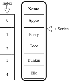
Apple, Berry, Coco, etc. are the values contained in this Series.
These values have their corresponding labels, which in this illustration
are simply numbers 0, 1, 2, and so on.
Collectively, these labels are called an index.
The data type of the values stored this Series is a string.
What is a DataFrame?
A DataFrame is a two-dimensional labeled data structure with columns of potentially different data types. A DataFrame is perfect for storing data in tabular format. Each column contain rows of the same length. The basic structure of a DataFrame is shown as follows:
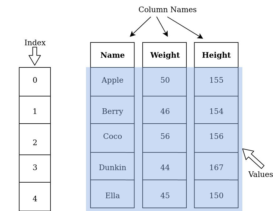
This DataFrame contains five rows (indexed by labels 0, 1, 2, …)
and three columns, labeled Name, Weight, and Height, respectively.
A DataFrame can be thought of as a collection of Series concatenated
side-by-side, where each column in a DataFrame is a Series object.
In the example above, there are three Series which are named
Name, Weight and Height.
Note that all columns in a DataFrame share a common index.
What Data Type?
Discuss with your neighbor (or colleague): What are the data types of
Name,Weight, andHeight?Solution
Nameclearly has a string data type. BothWeightandHeightare of numerical data type. Python makes a distinction of whole numbers (int, or integers) and real numbers that can contain a decimal point (float, short for floating point). While the numbers suggest in that particular table suggest that they can be represented by integers, we know from the real life that these better befloats because they can accommodate non-whole numbeers.
Several Helpful Analogies
Analogy to a spreadsheet—The DataFrame’s concept of a table with row and column labels is analogous to a spreadsheet (like Microsoft Excel, Google Sheet, etc.): Values in a spreadsheet is labeled by its column label (
A,B,C, …) and row number (1,2,3, …). An individual value, or cell in spreadsheet term, can be addressed by its corresponding column and row labels, such asA1,B27, etc. The same holds true for a DataFrame, by virtue of the column name and the index, as we will see later.Analogy to a database table—The vast majority of database systems today also store data in tabular format. A single row of a table is called a record, whereas a single value within a record (say, the
Namevalue in the illustration above) is often termed a field—that is the database’s analog of a column. In the example table above, there are 5 records, and each record has 3 fields (Name, Weight, and Height). The analogy with a database table actually goes stronger than that. In both DataFrame and database table, each column (field) has a specific data type. This data type is strictly enforced throughout the data operation (both reading and writing).
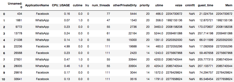
DataFrame Comprehension
Below is the screenshot of the Sherlock dataset that we will use in this lesson. From the figure below, answer the following:
- How many records and columns (fields) are in this DataFrame?
- What are the data types of each column?
- From the names of the columns, what are the meaning and purpose of each column?
Solution
The number of records is the number of the rows in the table, which is 10. The number of columns is 13, labeled
Unnamed: 0,ApplicationName, …,guest_time,Mem.It is obvious that most columns hold numerical values with the exception of
ApplicationName, which contains strings such ascminfltcolumn, which hold theNaNvalues.NaNstands for “not-a-number” (a special value of a real number on a computer, representing an invalid numerical value, such as the result of the division by zero, or a square-root of a negative number). pandas usesNaNto represent a missing value. In a latter section, we will distinguish the difference between integers (whole numbers) and real numbers (that have a decimal points).This table contains the record of resource utilization statistics gathered by the phone’s operating system. We will only explain the obvious ones here:
ApplicationName: the name of the application associated with this record;CPU_USAGE: the utilization level of the CPU, expressed in percentage (e.g.,100.0means the CPU is fully occupied with work);num_threads: the number of execution threads existing in the application (each thread executes a part of the program independently of the others);vsize: the size of the virtual memory allocated by the application;Mem: yet another measurement of memory usage.We will explain more fields in the lesson on machine learning. However, knowledge of computer and operating system architecture will be required to fully comprehend the meaning of these fields and their implications.
Working with Series
Now we begin a hands-on learning on pandas’ Series object.
We will first cover how to retrieve certain element(s) from a Series,
as well as how to update the values of these elements.
Creating a Series Object
A Series object can be created by feeding an input list to pandas.Series.
For example,
CPU_USAGE = pandas.Series([0.16, 0.07, 0.23, 0.24, 0.14, 4.99, 0.23, 0.47, 0.46, 0.17])
is a Series containing 10 measurements of the relative CPU usage of a computer.
We can use the print function to display the content of this object:
print(CPU_USAGE)
0    0.16
1    0.07
2    0.23
3    0.24
4    0.14
5    4.99
6    0.23
7    0.47
8    0.46
9    0.17
dtype: float64
The print out of CPU_USAGE shows the three key elements of a Series:
the values, the index (labels), and the data type.
Can you identify them from the output above?
The length of the Series object can be queried using the len function,
similar to list, dict, and other types of containers in Python:
print(len(CPU_USAGE))
10
Series can also be created from a Numpy array. For example:
# This creates an array of five even numbers:
numbers = numpy.arange(2,12,2)
print(numbers)
print()
# Now create a Series object that takes `numbers` as its values:
numseries = pandas.Series(numbers)
print(numseries)
[ 2  4  6  8 10]

0     2
1     4
2     6
3     8
4    10
dtype: int64
The first line of the output comes from printing numbers.
After converted to a Series, the data acquires an index.
Accessing Elements in a Series
Since a Series can contain many elements (values),
how can we access an individual element, or a group of elements?
Let us first learn how to read the element(s);
writing the elements will be discussed afterwards.
Accessing a Single Element
We can access an individual element in a Series by using the
[] array subscripting operator:
print(CPU_USAGE[3])
0.24
Array Subscripting or Array Indexing?
In many computer languages including Python, the
[]operator is famously used to subscript, or index, an array, that is, to refer to a specific element in the array by means of its position or its label. These two verbs (subscript and index) are used interchangeably in computer literature. Since the term index has a particular meaning in pandas, we will use the term subscript(ing) instead of index(ing) to refer to the action of the[]operator. We do this throughout this lesson to avoid confusion. The[]operator will be called the subscript operator.
On the surface this looks like the usual Python list or
Numpy ndarray, where individual elements are accessed
using an integer from 0, 1, 2, and so on.
But pandas use the labels stored in its index.
When we have a non-sequential index, then we have to access it
by the value of the label:
MEM_USAGE = pandas.Series([0.16, 0.07, 0.23, 0.24, 0.14],
                          index=[3, 1, 4, 2, 7])
print(MEM_USAGE)
3    0.16
1    0.07
4    0.23
2    0.24
7    0.14
dtype: float64
In this case, MEM_USAGE[3] will yield 0.16, not 0.24.
The element access of a Series behaves more like a dict
than like a regular array.
Accessing a Subset of a Series
With pandas, many elements can be accessed at once.
Continuing the MEM_USAGE example above:
print(MEM_USAGE[[1,3]])
1    0.07
3    0.16
dtype: float64
The result of this subsetting operation is actually
another Series object!
Subscripting with a Boolean Array
Accessing a Series with an array of Boolean (True or False) values
is a special case:
This subscripting operation acts as a “row selector”,
where the True values will select the corresponding elements.
The following example demonstrates the selection of elements:
print(MEM_USAGE[[True, False, False, True, True]])
3    2.00
2    0.24
7    0.33
dtype: float64
This gets to select the first, fourth, and fifth elements in MEM_USAGE.
Note that the length of the Boolean array needs to be the same as
the length of the Series.
This method of subscripting with a Boolean array
will come in handy in the next episode,
when we use certain logical criteria to filter the data.
Updating Elements in a Series
Now let us learn how to write (update) values into a Series.
The .loc[] operator provides a reliable mechanism to update
the values stored in a Series or DataFrame.
Whereas some write access is possible using the classic [] notation,
it is strongly recommended that we use the .loc[] operator.
Some non-working examples will be given later to demonstrate this point.
Updating a single element is as easy as an assignment operation:
print("Before update:")
print(MEM_USAGE[7])
print(MEM_USAGE.loc[7])
MEM_USAGE.loc[7] = 0.33
print("After update:")
print(MEM_USAGE.loc[7])
print(MEM_USAGE)
Before update:
0.14
0.14
After update:
0.33
3    0.16
1    0.07
4    0.23
2    0.24
7    0.33
dtype: float64
The first two output lines in the example above show
that for read access, both the [] and .loc[] operators
have the same effect.
We can also use .loc[] to set new values to a subset of the Series:
MEM_USAGE.loc[[1,3]] = [4, 2]
print(MEM_USAGE)
3    2.00
1    4.00
4    0.23
2    0.24
7    0.33
dtype: float64
The Boolean-array subscripting will also work to selectively update a subset of the values.
A
Seriesof ExerciseWhat are the contents of
MEM_USAGEafter each of the following assignments:MEM_USAGE.loc[[True, False, False, True, True]] = [ 1.0, 2.0, 3.0 ] print(MEM_USAGE)MEM_USAGE.loc[[True, False, False, True, True]] = 0 print(MEM_USAGE)
A
SeriesKind of ConfusionFor this challenge, please reset the values of
MEM_USAGEfirst:MEM_USAGE = pandas.Series([0.16, 0.07, 0.23, 0.24, 0.14], index=[3, 1, 4, 2, 7])What are the contents of
MEM_USAGEafter each of the following assignments (please do these assignments in order):MEM_USAGE[7] = 0.33 print(MEM_USAGE)MEM_USAGE[[1,3]] = [4, 2] print(MEM_USAGE)MEM_USAGE[[True, False, False, True, True]] = [ 1.0, 2.0, 3.0 ] print(MEM_USAGE)MEM_USAGE[[True, False, False, True, True]] = 0 print(MEM_USAGE)Which one(s) works correctly? Any assignment that produce surprising results?
The examples above show that updating
Serieselements using the[]operator does not always work as expected.
Readers who need a more definitive guideline on accessing
and manipulating elements in a Series are referred to
pandas guide to indexing and selecting data.
The key point is that accessing row(s) of a Series
(and later DataFrame)
can be safely done using the .loc[] operator.
The
.iloc[]operatorThe label-based element access is done using the
[]and.loc[]operators. These rely on the index of theSeries. It is also possible to do a position-based access using the.iloc[]operator, using the familiar integer values 0, 1, 2, … and so on. Consider again theMEM_USAGEseries:MEM_USAGE = pandas.Series([0.16, 0.07, 0.23, 0.24, 0.14], index=[3, 1, 4, 2, 7])In the underlying array that stores the data for
MEM_USAGE, the elements are indeed ordered in the way it was given above. The.iloc[]operator bypasses the index:print(MEM_USAGE.iloc[1], MEM_USAGE.iloc[2])0.07 0.23MEM_USAGE.iloc[2] = 27 print(MEM_USAGE)3 0.16 1 0.07 4 27.00 2 0.24 7 0.14 dtype: float64The
.iloc[]operator can also be used to reliably update elements of a series based on the position of the element.
Making a Copy
When working with a Series or DataFrame object,
sometimes we want to create a copy so that we can clobber
the copy without altering the original.
This can be easily done using the copy method.
MEM_USAGE = pandas.Series([0.16, 0.07, 0.23, 0.24, 0.14],
                          index=[3, 1, 4, 2, 7])
copy_usage = MEM_USAGE.copy()
copy_usage[3] = 1.23
print("Value in the copy:", copy_usage[3])
print("Value in the original:", MEM_USAGE[3])
Value in the copy: 1.23
Value in the original: 0.16
Contrast that to:
MEM_USAGE = pandas.Series([0.16, 0.07, 0.23, 0.24, 0.14],
                          index=[3, 1, 4, 2, 7])
alias_usage = MEM_USAGE
alias_usage[3] = 1.23
print("Value in the alias:", alias_usage[3])
print("Value in the original:", MEM_USAGE[3])
Value in the copy: 1.23
Value in the original: 1.23
In Python, variables are simply references to the actual objects.
Therefore making an assignment (alias_usage = MEM_USAGE)
simply makes a copy of the reference, not of the objects.
Working with DataFrames
Creating a DataFrame Object
A DataFrame object can be created in many ways.
If the data size is relatively small, it can be created from a list of lists
(i.e. nested list):
avatars = pandas.DataFrame([['Apple', 50, 155],
                            ['Berry', 46, 154],
                            ['Coco', 56, 156],
                            ['Dunkin', 44, 167],
                            ['Ella', 45, 150]],
                            columns=['Name', 'Weight', 'Height'])
In the example above, we are creating a DataFrame variable called
avatars to contain the information about the figures involved
in a computer game.
The first argument, a nested list, specifies the contents of the DataFrame.
The outer list contains five other lists, each of which contains
three elements—the name, weight (in kg), and height (in cm)
of the virtual person, in that order.
The second argument defines the names of the columns.
(Of necessity, the columns= argument name must be specified,
because it was specified as the third argument in
the syntax of pandas.DataFrame
call.)
We can inspect the contents of the DataFrame by printing the variable:
print(avatars)
     Name  Weight  Height
0   Apple      50     155
1   Berry      46     154
2    Coco      56     156
3  Dunkin      44     167
4    Ella      45     150
The first row of the printout shows the column names,
whereas the first column contains the index of the rows.
The default index is a zero-based integer sequence (0, 1, 2, …).
(As we will see later, the index and column name are used to
refer to a specific cell in the DataFrame,
much like the row and column numbers in a spreadsheet.)
Index in DataFrames
The index can be thought as a special column which hold the “labels” of the rows in a table. Using a given label, we can easily refer to its corresponding row in the table.
Just as the column names in a
DataFrame, the values of the index can also be defined to be anything, including string values. We could use this feature to work with meaningful names to refer to the particular columns and rows in the table, as opposed to using row and column numbers. For example, if a table contain four rows representing data from each season, it is more sensible to assignSpring,Summer,Fall,Winteras the row names than having to remember that0refers toSpring,1toSummer, etc.In the next episode, we will learn that pandas itself will assign meaningful values to the
DataFrameobjects it produces from certain type of operation (for example, when computing mean values after grouping the data according to certain criteria).
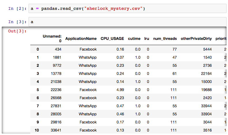
Tabular Output in Jupyter Notebook
Jupyter notebook has a nice tabular output for DataFrame objects. Simply type the variable name and press Enter to view the output. For the example above:
The column names and index are printed in boldface. When the table is large (has many records and/or columns), the Jupyter interface will allow you to scroll the page horizontally and/or vertically to inspect the contents of the entire table. Here is an example of screenshot from a dataset which we will encounter shortly:
How Big is My Data?
Once a DataFrame is created, we can know its properties by using various
functions and attributes.
We will learn some of these here.
The len function can be used to get the number of rows in a DataFrame:
print(len(avatars))
But a DataFrame has another dimension—the number of columns.
We can inquire both the numbers of rows and columns using the shape
attribute:
print(avatars.shape)
(5, 3)
The shape attribute yields a tuple of two numbers:
the number rows and the number of columns.
print("The number of rows =", avatars.shape[0])
print("The number of columns =", avatars.shape[1])
An attribute should not be called with the () operator.
In fact, that will trigger an error in Python.
But because shape returns a tuple, which is an array-like object,
we use the [] subscript operator to get the individual value.
The values of the index (i.e. the row labels) can be queried too:
print(avatars.index)
RangeIndex(start=0, stop=5, step=1)
The index attribute returns a special index object called RangeIndex,
which means a regular sequence of numerical labels,
starting from 0 and ending just before 5
(the usual Python endpoint convention), with an increment of 1.
This index is also an array-like object–give it a try.
The column names are given by the columns attribute:
print(avatars.columns)
Index(['Name', 'Weight', 'Height'], dtype='object')
Like the shape attribute, the column attribute is also array-like,
meaning that you can get the individual element using the []
subscript operator.
Incidentally, the columns attribute returns an Index object—although
we don’t customarily call the collection of the column names an “index”.
Finally, the data types of the columns can be queried using the dtypes attribute:
print(avatars.dtypes)
Name      object
Weight     int64
Height     int64
dtype: object
We will discuss data types more in depth later.
Column Name Exercise
How to print the name of the second column of
avatars?Solution
print(avatars.columns[1])Weight
Is it a
Seriesor aDataFrame?At times, we may want to know whether an object is a
Seriesor aDataFrame. This may be true when we work with a large number of objects, or when we are not clear about the result of an operation.We have created a number of objects so far. Now, find out the type of
CPU_USAGEandavatars!Solution
print(type(CPU_USAGE))
print(type(avatars))
<class 'pandas.core.series.Series'> <class 'pandas.core.frame.DataFrame'>
Other Ways of Constructing a DataFrame
There are many other ways to construct a
DataFrameobject. The same avatars DataFrame can also be created using the dict-of-list argument:avatars_alt = pandas.DataFrame({'Name': ['Apple', 'Berry', 'Coco', 'Dunkin', 'Ella'], 'Weight': [50, 46, 56, 44, 45], 'Height': [155, 154, 156, 167, 150]}, column=['Name', 'Weight', 'Height'])This alternative way is suitable if the input data is already laid out in a column-by-column fashion. The input arrays can be lists (like the example above), Numpy arrays, or other array-like objects.
Caveat: The second argument (
column=) above is needed to enforce the order of the column. In newer pandas (version 0.23 and later) and Python (3.6 and later), the order given above will be respected by pandas, but in older versions the column order is not guaranteed.A DataFrame object can also be created from a two-dimensional Numpy array or another DataFrame object as its data source. Please refer to the reference documentation of
pandas.DataFrame.
Exercise: Creating a DataFrame object
Create the
App_infoDataFrame whose contents are as follows:print(App_info)ApplicationName CPU_USAGE vsize 0 Facebook 0.16 2204700672 1 WhatsApp 0.07 1992155136 2 WhatsApp 0.23 2008158208 3 WhatsApp 0.24 2059481088 4 WhatsApp 0.14 2020352000 5 Facebook 4.99 2272055296 6 Facebook 0.23 2275667968 7 WhatsApp 0.47 2085740544 8 WhatsApp 0.46 2085740544 9 Facebook 0.17 2276429824Extra challenge: change the index of
App_infoto a letter sequence (a,b,c, …j).Hint: Re-create
App_infowith the appropriate index, or alter theindexattribute of the existingApp_infoobject.
Reading Data from a File
One of Pandas’ strengths is its ability to read and write data
in many different formats.
A popular format for tabular data is “CSV” (shorthand for comma-separated values).
A CSV data is stored in a plain text file,
very much like the two-dimensional tabular format of a DataFrame:
Each text line represents a record (row), and
each line contains one or more values separated by the comma (,) character.
A CSV file which contains the data of the avatars DataFrame
introduced earlier would look like this
(see avatars.csv in the hands-on directory for this training module):
Name,Weight,Height
Apple,50,155
Berry,46,154
Coco,56,156
Dunkin,44,167
Ella,45,150
The first line usually contains the column names. In this case, we do not store the index, because we use pandas’ default choice.
We use the pandas.read_csv function to load the CSV data into a DataFrame object:
avatars_read = pandas.read_csv("avatars.csv")
The read_csv function provides a lot of control on
how to read the CSV data.
It can deal with variations in the CSV format
(i.e. if the value separator is not a comma),
determine the column names, how many records to read,
selecting which columns to retain in the output, defining column names, and many more.
We will use some of these capabilities in this lesson.
Refer to the
Pandas documentation on read_csv
for complete information.
Loading Sherlock Data
We begin our foray into the Sherlock’s “Applications” dataset
by loading a tiny subset of the data from a CSV file named sherlock_mystery.csv,
located in the sherlock subdirectory.
Let us read the data into a Python variable named df_mystery.
Starting Small
The Sherlock sample dataset contains a very large CSV file named
Applications.csv, containing nearly 15 million rows of observations collected on an Android smartphone. We will be using this data throughout this lesson as well as the subsequent Machine Learning and Deep Learning lessons. It is imperative that we gain familiarity with this dataset, so that we can design a sensible approach to detect running applications on the phone, as stated at the beginning of this module.To help learners gradually gain familiarity and confidence in working with large datasets, we have prepared subsets of the original data with increasing levels of size and complexity. In the Big Data lesson, we will start by loading a tiny sample dataset (
sherlock_mystery.csv), then continue with a medium-sized table (sherlock_mystery_2apps.csv). In the Machine Learning and Deep Learning lessons we will encounter larger and more complex tables.
Reading
sherlock_mystery.csvUse
pandas.read_csvto read in the data file. Name the variabledf_mystery. Print the dataset. How many columns and rows exist in this dataset?(Remember that Jupyter users have an option to display the
DataFramein a nice format by simply typing the variable name.)Solution
df_mystery = pandas.read_csv('sherlock/sherlock_mystery.csv')
print(df_mystery)
(The
sherlock/subdirectory may or may not be necessary—check your current working directory by thepwdmagic command.)The printout is very long—we will truncate the output manually here:
     Unnamed: 0 ApplicationName  CPU_USAGE  cutime  lru  num_threads  \
0           434        Facebook       0.16     0.0    0           77
1          1881        WhatsApp       0.07     1.0    0           47
2          9772        WhatsApp       0.23     0.0    0           55
3         13778        WhatsApp       0.24     0.0    0           61
4         21038        WhatsApp       0.14     1.0    0           55
5         22236        Facebook       4.99     0.0    0          111
6         26568        Facebook       0.23     0.0    0          111
7         27831        WhatsApp       0.47     1.0    0           55
8         28005        WhatsApp       0.46     1.0    0           55
9         29816        Facebook       0.17     0.0    0          111
10        33641        Facebook       0.13     0.0    0          111
(output truncated)
..          ...             ...        ...     ...  ...          ...
(output truncated)
190      752526        Facebook       0.39     0.0    0           18
191      762346        Facebook       0.60     0.0    0          178
192      765532        Facebook       0.52     0.0    0          178
193      767094        Facebook       0.16     0.0    0           18
194      771734        WhatsApp       0.27     1.0    0           65
195      776470        Facebook       0.40     0.0    0          178
196      776474        WhatsApp       0.26     1.0    0           57
197      779599        Facebook       0.39     0.0    0          178
198      784035        Facebook       0.15     0.0    0           18
199      786781        WhatsApp       0.24     3.0   15           48

(more output truncated)

[200 rows x 14 columns]
At the end of a long, truncated DataFrame output, the number of rows and columns are printed.
What do we learn from the exercise of reading and printing
the sherlock_mystery.csv data?
While the data is far from being big (the CSV file size is less than 20 kilobytes),
it is certainly not comfortable for point-by-point inspection
or manual manipulation.
It has more than 100 rows and 10 columns.
A DataFrame in pandas has a lot of powerful utilities to extract knowledge
from a dataset; we will learn a few of these now.
Initial Exploration: head, tail, describe, info
It is customary to inspect only a fraction of the data
at the beginning and the ending of the rows.
The head and tail method does precisely that.
# Load sherlock_mystery.csv data onto `df_mystery` first!

# Prints the first 10 rows of `df_mystery`
print(df_mystery.head(10))
   Unnamed: 0 ApplicationName  CPU_USAGE  cutime  lru  num_threads  \
0         434        Facebook       0.16     0.0    0           77
1        1881        WhatsApp       0.07     1.0    0           47
2        9772        WhatsApp       0.23     0.0    0           55
3       13778        WhatsApp       0.24     0.0    0           61
4       21038        WhatsApp       0.14     1.0    0           55
5       22236        Facebook       4.99     0.0    0          111
6       26568        Facebook       0.23     0.0    0          111
7       27831        WhatsApp       0.47     1.0    0           55
8       28005        WhatsApp       0.46     1.0    0           55
9       29816        Facebook       0.17     0.0    0          111

   otherPrivateDirty  priority   utime       vsize  cminflt  guest_time  \
0               5444        20   466.0  2204700672      NaN   21.024754
1               1540        20   358.0  1992155136      NaN   12.870721
2               2736        20  3463.0  2008158208      NaN  170.070837
3              22164        20  5244.0  2059481088      NaN  257.714198
4              15000        20  1351.0  2020352000      NaN   66.011599
5              19688        14   460.0  2272055296      NaN   17.092659
6               2420        14  1243.0  2275667968      NaN   59.467658
7              33944        20  4200.0  2085740544      NaN  205.777315
8              33904        20  4204.0  2085740544      NaN  207.103771
9               3044        14  1572.0  2276429824      NaN   74.294757

          Mem       queue
0  2204700672  100.000000
1  1992155136  100.000000
2  2008158208  100.000000
3  2059481088  100.000000
4  2020352000  100.000000
5  2272055296  121.428571
6  2275667968  121.428571
7  2085740544  100.000000
8  2085740544  100.000000
9  2276429824  121.428571
print(df_mystery.tail())
# This is the same as print(df_mystery.tail(5))
     Unnamed: 0 ApplicationName  CPU_USAGE  cutime  lru  num_threads  \
195      776470        Facebook       0.40     0.0    0          178
196      776474        WhatsApp       0.26     1.0    0           57
197      779599        Facebook       0.39     0.0    0          178
198      784035        Facebook       0.15     0.0    0           18
199      786781        WhatsApp       0.24     3.0   15           48

     otherPrivateDirty  priority    utime       vsize  cminflt  guest_time  \
195              75104        20  11020.0  2483150848      0.0  545.926305
196              15840        20   6938.0  2094870528    501.0  344.944906
197              78648        20  11714.0  2482655232      0.0  584.140036
198               2916        20   5450.0  2123321344      0.0  267.732926
199               3300        20   1877.0  1993637888   1021.0   89.041681

            Mem  queue
195  2483150848  100.0
196  2094870528  100.0
197  2482655232  100.0
198  2123321344  100.0
199  1993637888  100.0
Without an argument, head and tail will yield the first or last five records.
The head or tail method returns a new DataFrame
that contains a subset of the original df_mystery.
The row labels (index) are preseved by these methods.
pandas can compute descriptive statistics for all the numerical columns by
using the describe method:
df_mystery.describe()
          Unnamed: 0   CPU_USAGE      cutime        lru  num_threads  \
count     200.000000  200.000000  200.000000  200.00000   200.000000
mean   400417.440000    0.224750    0.420000    0.07500    71.365000
std    236324.977496    0.417532    0.926223    1.06066    45.599543
min       434.000000    0.000000    0.000000    0.00000    11.000000
25%    191892.750000    0.080000    0.000000    0.00000    49.000000
50%    390047.500000    0.160000    0.000000    0.00000    62.000000
75%    626675.250000    0.270000    0.000000    0.00000    98.750000
max    786781.000000    4.990000    4.000000   15.00000   190.000000

       otherPrivateDirty    priority         utime         vsize      cminflt  \
count          200.00000  200.000000    200.000000  2.000000e+02   152.000000
mean         20426.28000   19.730000   4224.705000  2.175793e+09   297.631579
std          23323.22431    1.146154   5493.086456  1.417478e+08   418.205496
min             32.00000   14.000000     23.000000  1.983623e+09     0.000000
25%           2826.00000   20.000000    559.750000  2.095809e+09     0.000000
50%          13552.00000   20.000000   2238.500000  2.107628e+09     0.000000
75%          29993.00000   20.000000   6457.000000  2.252854e+09   513.000000
max         114972.00000   20.000000  34615.000000  2.633560e+09  1550.000000

        guest_time           Mem       queue
count   200.000000  2.000000e+02  200.000000
mean    207.781320  2.175793e+09  100.910714
std     274.703022  1.417478e+08    3.926164
min      -4.436543  1.983623e+09  100.000000
25%      24.585457  2.095809e+09  100.000000
50%     109.155168  2.107628e+09  100.000000
75%     318.810321  2.252854e+09  100.000000
max    1725.901364  2.633560e+09  121.428571
The describe() output is a dizzying table of numbers,
but these numbers tell a lot of story about the data!
For every column, pandas compute eight values:
-
The first three lines show the count of the data points (more precisely: the number of non-missing data points), the mean and standard deviations (
std).stdgives the measure of the variability of the individual data points around the mean value. -
The next five line covers the minimum, the 25%, 50%, 75% percentile, (also known as the first quartile, median, third quartile), and the maximum values, respectively. These numbers give the sense of the range of the values (from minimum to maximum values) and a different way to measure the spread of the data points.
It is worth taking time to comprehend these statistics. Right away we have several observations:
-
The
cminflthas only 152 values. Why is that? There are 48 rows in the dataset that are missing the values for this column. Pandas can handle missing values gracefully. We will discuss this issue in a latter episode. -
The
cutimecolumn hasstdthat is greater thanmean. Further examining the quartile values, we suspect that most of the time the value ofcutimeis zero—except on very few instances. Contrast this with the statistics of thevsizecolumn: the values vary between 1.98 and 2.63 billions.
At the end of this episode we will return to these statistics and use visualization to comprehend them better.
pandas computes statistics only for numeric columns
The ApplicationName column did not appear in the output above
because its data type not text, not numbers.
About pandas Object-Oriented Interface
pandas uses an object-oriented (OO) application programming interface (API). In this approach, the functions that operate on the object are called methods, and the object being operated upon is specified before the method, separated by a period (
.). Considerdf_mystery.head(10)as an example: the input objectdf_mysteryis specified before theheadfunction. Additional arguments for the function is after the function name, between the parentheses, just like any other Python functions.An attribute of an object is a special “variable” belonging to that object. For example,
shapeandcolumnsdemonstrated above. To read an attribute, simply give the object name before the attribute name, but do not append(). Some attributes can be written (updated). For example, we can change the names of the columns by assigning a new array of strings to thecolumnsattribute.
The OO notation allows for convenient chained operation—which we will be using extensively with Pandas. Consider the following:
print(df_mystery.tail(5).index)
RangeIndex(start=195, stop=200, step=1)
First, df_mystery.tail(5) is computed (on the fly).
This returns a new DataFrame, as it was previously discussed.
Then we query the index of the new DataFrame using the index method.
It is important to keep in mind that the chained operations
occur sequentially from left to right.
Statistics of a Tail
What is the meaning of
df_mystery.tail(5).describe()? Examine its output and compare it with the statistics gathered for the entiredf_mysteryprinted earlier.
Printing the Middle Rows
Create a Python statement to return a subset of
df_mysterywith row labels10through19(inclusive). (Hint: combineheadandtailmethods.)Extra challenge: Compute the statistics of that middle rows using the
describemethod.
Finally, the info() DataFrame method provides a brief summary
about a DataFrame object:
- the information about the index
- the information about every column (the name, the number of non-null elements, and the data type)
df_mystery.info()
<class 'pandas.core.frame.DataFrame'>
RangeIndex: 200 entries, 0 to 199
Data columns (total 14 columns):
Unnamed: 0           200 non-null int64
ApplicationName      200 non-null object
CPU_USAGE            200 non-null float64
cutime               200 non-null float64
lru                  200 non-null int64
num_threads          200 non-null int64
otherPrivateDirty    200 non-null int64
priority             200 non-null int64
utime                200 non-null float64
vsize                200 non-null int64
cminflt              152 non-null float64
guest_time           200 non-null float64
Mem                  200 non-null int64
queue                200 non-null float64
dtypes: float64(6), int64(7), object(1)
memory usage: 22.0+ KB
To conclude this section of the initial data exploration:
- The
infomethod provides a summary about the key properties of a DataFrame object (not so much about the data it contains); - The
describemethod provides a statistical summary of the various numerical columns in the DataFrame; - The
headandtailprovide “sneak peek” of the data at the beginning and end of the table, respectively.
Data Types
Let us now revisit the matter of data type in pandas,
as this is an important concept to understand and apply while working with data.
We start with the example of df_mystery:
print(df_mystery.dtypes)
Unnamed: 0             int64
ApplicationName       object
CPU_USAGE            float64
cutime               float64
lru                    int64
num_threads            int64
otherPrivateDirty      int64
priority               int64
utime                float64
vsize                  int64
cminflt              float64
guest_time           float64
Mem                    int64
queue                float64
dtype: object
The dtypes attribute returns the data type of each column.
Data type is an important property of every element of the Series
and DataFrame objects.
Pandas supports the following common Python data types:
strfor strings (text data).intfor integers ranging from approximately –9.2 × 10¹⁸ to 9.2 × 10¹⁸. This is equivalent to Numpy’sint64, which is a 64-bit integer data type. An integer, by definition, does not have any decimal point.floatfor real numbers (with decimal points) with magnitudes ranging from approximately ±2.23×10-308 to ±1.80×10308. This is equivalent to Numpy’sfloat64, which is a 64-bit floating-point data type.
There are other data types which we will not discuss here:
-
For numerical values, there are numbers with other precisions (like 2- or 4-byte integers or 32-bit real numbers).
-
There is also a
'datetime64'data type with resolution of nanoseconds: columns in a CSV file that contain date/time data can be loaded onto aDataFramewith an appropriate converter or data type specification. Interested readers can learn more by consulting pandas guide to time series / date functionality. -
Many string-valued columns actually contain categorical data, because they contain only a limited set of values. Significant efficiency can be gained by using
'categorical'to represent such data. Refer to pandas guide to categorical data to get started.
Returning to the example of df_mystery.dtypes above,
we see many columns have either the int64 or float64 data types,
as expected for these numerical quantities.
The exception is ApplicationName, whose type is called object—referring
to a generic Python object.
The values contained in this column are strings (such as 'WhatsApp',
'Gmail', 'Waze', etc.).
Indeed, because strings are of unpredictable lengths,
pandas was forced to use the most generic object representation.
The Importance of Data Types
It is important that each column in a
DataFramehas the appropriate data type for its values. Fortunately, in many instances pandas can deduce the data types automatically. For example, when constructing theavatarsDataFrame above, pandas knows thatWeightandHeightcolumns contain whole numbers, therefore they will have theint64data type. Similarly, whenpandas.read_csvreads data from a CSV file, it will scan the (initial) contents of the file to deduce the most appropriate data type for each column.In real life, there are cases where
pandas.read_csvwill fail to predict the most appropriate data type. To address this issue, we need to specify the optionaldtypeargument when callingread_csv. In some of our hands-on activities we will do this to enforce the data type correctness. Thedtypespecification will forceread_csvto validate the values of the input data. For example, when reading in thenum_threadscolumn, all numbers must be integers—it is not valid to have2.5as a value here.pandas.read_csvwill raise an error when such an invalid value is encoutered. When working with real data and real-life problem, it is advisable to always use thedtypeargument to ensure that all columns have the correct data types.
Data Type of What?
When working with a
Seriesor aDataFrame, the term data type usually refers to that of the values contained in theSeriesorDataFrameobject. BothSeriesandDataFrameare examples of containers. A container which is a Python object that contains other objects.This is not to be confused with the class of the Series object itself, which we can query using the
typefunction:print(type(MEM_USAGE))<class 'pandas.core.series.Series'>Indeed,
pandas.Seriesis just an alias topandas.core.series.Series. The former is the public API, whereas the latter is the internal implementation API.
pandas.core.series.Seriesis the type of the container object, whereas the values contained within this container can be strings, orint64s, and so on.
Accessing Elements in a DataFrame
Now let us learn how to access an individual element or a group of elements
in a DataFrame object.
This is an extension of the similar discussion for Series.
Since DataFrame can be viewed as a collection of Series objects
sharing a common index, many of the techniques described there apply here.
But because this is a two-dimensional object, there needs to be a way to
access both axes (the rows as well as the columns).
The [] Operator
The classic [] operator can be used to access a particular column, such as:
df_mystery['ApplicationName']
0      Facebook
1      WhatsApp
2      WhatsApp
3      WhatsApp
4      WhatsApp
5      Facebook
6      Facebook
7      WhatsApp
8      WhatsApp
9      Facebook
...
190    Facebook
191    Facebook
192    Facebook
193    Facebook
194    WhatsApp
195    Facebook
196    WhatsApp
197    Facebook
198    Facebook
199    WhatsApp
Name: ApplicationName, Length: 200, dtype: object
Use the type function to find out the type of this object:
print(type(df_mystery['ApplicationName']))
<class 'pandas.core.series.Series'>
It is a Series!
Multiple columns can be retrieved by passing a list of the column names to the subscript operator:
print(df_mystery[['ApplicationName', 'CPU_USAGE', 'num_threads']])
    ApplicationName  CPU_USAGE  num_threads
0          Facebook       0.16           77
1          WhatsApp       0.07           47
2          WhatsApp       0.23           55
3          WhatsApp       0.24           61
4          WhatsApp       0.14           55
5          Facebook       4.99          111
6          Facebook       0.23          111
7          WhatsApp       0.47           55
8          WhatsApp       0.46           55
9          Facebook       0.17          111
..              ...        ...          ...
190        Facebook       0.39           18
191        Facebook       0.60          178
192        Facebook       0.52          178
193        Facebook       0.16           18
194        WhatsApp       0.27           65
195        Facebook       0.40          178
196        WhatsApp       0.26           57
197        Facebook       0.39          178
198        Facebook       0.15           18
199        WhatsApp       0.24           48

[200 rows x 3 columns]
From the output, it is quite obvious that
selecting multiple columns at once will return
a DataFrame.
Filtering Rows—We can also feed an array of Boolean to the [] operator;
but unlike the two previous uses, we will select rows (instead of columns)
based on the Boolean values.
Selecting Rows
Try the following code and explain your observation:
df6 = df_mystery.head(6)
df6_filt = df6[[True, False, False, True, True, False]]
print(df6)
print(df6_filt)
Solution
The second
   Unnamed: 0 ApplicationName  CPU_USAGE  cutime  lru  num_threads  \
0         434        Facebook       0.16     0.0    0           77
3       13778        WhatsApp       0.24     0.0    0           61
4       21038        WhatsApp       0.14     1.0    0           55

   otherPrivateDirty  priority   utime       vsize  cminflt  guest_time  \
0               5444        20   466.0  2204700672      NaN   21.024754
3              22164        20  5244.0  2059481088      NaN  257.714198
4              15000        20  1351.0  2020352000      NaN   66.011599

          Mem  queue
0  2204700672  100.0
3  2059481088  100.0
4  2020352000  100.0
The resulting DataFrame has three rows, corresponding to the selection made by the Boolean array above.
The .loc[] Operator
We can retrieve one or more rows of data using
the .loc[] operator, as with the Series:
print(df_mystery.loc[1])
Unnamed: 0                 1881
ApplicationName        WhatsApp
CPU_USAGE                  0.07
cutime                        1
lru                           0
num_threads                  47
otherPrivateDirty          1540
priority                     20
utime                       358
vsize                1992155136
cminflt                     NaN
guest_time              12.8707
Mem                  1992155136
queue                       100
Name: 1, dtype: object
This returns a Series object.
And lo and behold, the index of this object
contains the column names!
You can also return multiple rows, e.g.
print(df_mystery.loc[[1,3,5]])
   Unnamed: 0 ApplicationName  CPU_USAGE  cutime  lru  num_threads  \
1        1881        WhatsApp       0.07     1.0    0           47
3       13778        WhatsApp       0.24     0.0    0           61
5       22236        Facebook       4.99     0.0    0          111

   otherPrivateDirty  priority   utime       vsize  cminflt  guest_time  \
1               1540        20   358.0  1992155136      NaN   12.870721
3              22164        20  5244.0  2059481088      NaN  257.714198
5              19688        14   460.0  2272055296      NaN   17.092659

          Mem       queue
1  1992155136  100.000000
3  2059481088  100.000000
5  2272055296  121.428571
To access a particular element,
the .loc[] operator supports two arguments:
the row and column labels.
print(df_mystery.loc[1, 'num_threads'])
47
One or both of the argument(s) to the .loc[] operator
can also be an array of row/column labels.
For example:
df_mystery.loc[[1,2,5], ['num_threads', 'CPU_USAGE', 'ApplicationName']]
   num_threads  CPU_USAGE ApplicationName
1           47       0.07        WhatsApp
2           55       0.23        WhatsApp
5          111       4.99        Facebook
Similarly, an array of Boolean values can be given to select the row(s) and/or column(s).
print(df_mystery.loc[[False,True,True,False,True],
                     ['num_threads', 'CPU_USAGE']])
   num_threads  CPU_USAGE
1           47       0.07
2           55       0.23
4           55       0.14
What happen to the rest of the rows?
Well, as it turns out, if the length of the Boolean array
is too short compared to the number of rows (or columns),
then the rest of the elements are NOT selected
(i.e. they default to False).
For the array-like parameter, there is a special notation
to refer to “all the rows” or “all the columns”.
Simply feed a single colon (:) to the appropriate place,
then all the rows or columns will be included.
Slicing Operator
In Python, the colon operator is called slicing operator, allowing us to access (read/update) a subset of data specified by the beginning and/or ending label. Important! The rules for slicing in pandas are not identical to Python traditional slicing. For example, to retrieve rows with labels from 10 through 20, we use:
df_mystery.loc[10:20]Unnamed: 0 ApplicationName CPU_USAGE cutime lru num_threads \ 10 33641 Facebook 0.13 0.0 0 111 11 40917 Facebook 0.02 0.0 0 11 12 42067 Facebook 0.19 0.0 0 134 13 45601 Facebook 0.19 0.0 0 134 14 51672 Facebook 0.00 0.0 0 12 15 63332 Facebook 0.24 0.0 0 142 16 74881 Facebook 0.09 0.0 0 81 17 82073 Facebook 0.08 0.0 0 87 18 83528 WhatsApp 0.17 3.0 0 61 19 87373 Facebook 0.08 0.0 0 88 20 97640 WhatsApp 0.44 0.0 0 60 ... (output truncated)Any rows in between the two labels, including both endpoints, will be returned. Either the beginning or ending label or both can be omitted, in which case the result will start from the first row, or extend to the very last row of the dataset. The rules become tricky when one or the two labels are not found in the index. Please review them in pandas’ User Guide on Indexing and Selecting Data. Suffice it is to say that the safest way to use slicing operator in pandas is to specify only label(s) that exist on the DataFrame index, or omit one or two of the endpoints.
DataFrameandSeriesSubscripting ExercisesExercise 1 What does each expression below evaluate to? In other words, if you print them, what will be the output? Think first before you try them.
df_mystery.loc[1, :]
df_mystery.loc[:, 'CPU_USAGE']
Exercise 2 For each pair of commands below, what are the difference(s) within each pair? Print the first few elements of the result.
df_mystery['CPU_USAGE'] df_mystery[['CPU_USAGE']]df_mystery.loc[1] df_mystery.loc[[1]]Exercise 3 Given a DataFrame defined below:
D = [['Facebook', 0.16, 0.0, 77, 20],
     ['WhatsApp', 0.07, 1.0, 47, 20],
     ['WhatsApp', 0.23, 0.0, 55, 20],
     ['WhatsApp', 0.24, 0.0, 61, 20],
     ['WhatsApp', 0.14, 1.0, 55, 20]]

DF = pandas.DataFrame(D, columns=['AppName', 'CPU_USAGE', 'cutime',
                                  'num_threads', 'priority'])
which command(s) below give the following output:
    AppName  CPU_USAGE  num_threads
0  Facebook       0.16           77
1  WhatsApp       0.07           47
2  WhatsApp       0.23           55
3  WhatsApp       0.24           61
4  WhatsApp       0.14           55
DF[[0, 1, 3]]DF[['AppName', 'CPU_USAGE', 'num_threads']]DF.loc[['AppName', 'CPU_USAGE', 'num_threads']]DF[[True, True, False, True, False]]DF.loc[:, ['AppName', 'CPU_USAGE', 'num_threads']]Exercise 4 Try these commands to understand how the slicing works
df_mystery.loc[:10]
df_mystery.loc[:10, 'ApplicationName':'num_threads']
df_mystery.loc[20:]
df_mystery.loc[:]
MEM_USAGE.loc[:4]
MEM_USAGE.loc[2:]
Creative Challenges
The first column named
Unnamed: 0seems to contain absurd data. Using the subscripting syntax we’ve learned, create a new DataFrame that does not contain this column.Hint: There are a few ways of doing this, but there is one syntax that is particularly compact.
A Few Important Notes
The
.loc[]operator is the only way to select specific row(s) by their labels, as the[]operator is reserved to select only column(s).The
.iloc[]operator is also available to retrieve/update the row(s) of data by their positions.The
.loc[]and.iloc[]operators can be used to update the values at the specified location(s) in theDataFrame.To those who are used with the C/C++ or Python language: Use the two-argument subscripting syntax to safely update the
DataFramecontents:df_mystery.loc[2, 'CPU_USAGE'] = 1.00Do not use the nested subscript syntax that is commonly practiced in some languages:
df_mystery.loc[2]['CPU_USAGE'] = 1.00 ### BAD!df_mystery['CPU_USAGE'][2] = 1.00 ### BAD!
Summary of Subscripting Syntax
The subscript syntax on Series and DataFrame can be
overwhelming and confusing to new learners.
Here is a little table of the various syntax we have seen so far,
to summarize our learning:
For a Series variable called S:
| Syntax | Meaning |
|---|---|
S[ROW_SELECTOR] |
Read elements of the selected row(s) |
S.loc[ROW_SELECTOR] |
Read elements of the selected row(s) |
S.loc[ROW_SELECTOR] = NEW_VALS |
Update elements of the seleted rows(s) |
For a DataFrame variable called df:
| Syntax | Meaning |
|---|---|
df[COL_SELECTOR] |
Select (read) the specified column(s) |
df[ROW_BOOLEAN_SELECTOR] |
Select (read) the specified row(s) based on an array of Boolean values [1] |
df.loc[ROW_SELECTOR] |
Select (read) the specified row(s) |
df.loc[ROW_SELECTOR, COL_SELECTOR] |
Select (read) elements from the specified row(s) and column(s) |
df[COL_SELECTOR] = NEW_COL_VALS |
Update the selected column(s) with new values |
df.loc[ROW_SELECTOR] = NEW_ROW_VALS |
Update the selected rows(s) with new values |
df.loc[ROW_SELECTOR, COL_SELECTOR] = NEW_VALS |
Update elements on the specified row(s) and column(s) with new values |
For brevity, we omit the .iloc[] subscripting method from the tables.
ROW_SELECTOR can be one of the following:
-
A single row label
-
An array of row labels
-
An array of Boolean values (also referred to above as
ROW_BOOLEAN_SELECTOR) -
A literal
:character to indicate all rows
Similarly, COL_SELECTOR can be one of the following:
-
A single column name
-
An array of column names
-
An array of Boolean values
-
A literal
:character to indicate all columns
[1] Remember that df[BOOLEAN_ARRAY] will select rows, not columns.
This is an exception to the other general rules.
pandas user’s guide has a
comprehensive documentation
on selecting and indexing (subscripting) data,
which provides an authoritative guide on this subject matter.
Making Sense of Data with Visualization
Now that we have learn some basic skills on Series and DataFrame,
let us try one more exercises to familiarize ourselves
with the mystery of Sherlock data.
We will also make use of visualization here;
a latter episode will be dedicated to more in-depth visualization techniques.
Statistics of a Column
The
describeoperation also works on aSeriesobject. Print the descriptive statistics of just theCPU_USAGEcolumn.Solution
print(df_mystery['CPU_USAGE'].describe())count 200.000000 mean 0.244250 std 0.457354 min 0.000000 25% 0.087500 50% 0.160000 75% 0.270000 max 4.990000 Name: CPU_USAGE, dtype: float64
Let us look more closely into the statistics of one column:
print(df_mystery['vsize'].describe())
count    2.000000e+02
mean     2.175793e+09
std      1.417478e+08
min      1.983623e+09
25%      2.095809e+09
50%      2.107628e+09
75%      2.252854e+09
max      2.633560e+09
Name: vsize, dtype: float64
As we mentioned earlier, the quantities returned by the describe method
collectively make up the descriptive statistics about this data.
These numbers speak the range of the values, the mean and median,
as well as the spread of the data around the mean and median values.
For many people, it is much easier to “see” these values in a graph.
Therefore let us turn to visualization to help put the statistics in perspective.
First let us plot the raw values of vsize.
There is a built-in plotting utility in pandas to do so.
df_mystery['vsize'].plot(kind='line')
This statement asks pandas to print an (x–y) plot; by default two nearby data points are connected by lines. On a Jupyter notebook, the plot will be displayed inline when the code above is executed:
![Plot of df_mystery['vsize'] series](../fig/plot_line_mystery_vsize.png)
(On a terminal-based ipython or python session,
the plot will be displayed as a pop-up window.)
The y values are the values in the Series,
whereas the x values are the labels in the index.
The 1e9 printed on top of the graph by the vertical axis means that
the y-tick labels are to be multiplied by 109
(for example, the label 2.6 stands for 2.6 billions).
Verify that the minimum and maximum values correspond to the
output of the describe method above.
Descriptive statistics can also be visualized.
For massive amount of data the raw data plot would be very confusing:
imagine plotting 1,000,000 points as on a single plot like that?
The following is the code and output for a box plot for the vsize data:
seaborn.boxplot(x=df_mystery['vsize'], color='cyan')
![Box plot of df_mystery['vsize']](../fig/plot_box_mystery_vsize_cyan.png)
What is a box plot, or box-and-whisker plot?
A box plot is a method for graphically depicting groups of numerical data through their quartiles. The box extends from the Q1 to Q3 quartile values of the data, with a line at the median (Q2). The whiskers extend from the edges of box to show the range of the data. The position of the whiskers is set by default to a maximum of 1.5×IQR (where IQR = Q3 – Q1) from the edges of the box. Outlier points are those past the end of the whiskers. (Source: pandas manual page on
pandas.Series.plot.box).
Khan academy has a video that explains all the parts of a box-and-whisker plot.
The center line and edges of the box corresponds to the
25%, 50%, and 75% of the descriptive statistics.
The whisker on each side of the box is inteded to show
the range of the values from the minimum (maximum) to the Q1 (Q3).
However, if some points lie too far out
(beyond 1.5×IQR of the nearest quartile),
those points are deemed to be “outliers”, thus shown individually.
The graph above shows that the distribution of the value is skewed such that the values to the left of the median are more densely packed.
Let us compare this with the box plot for cutime:
print(df_mystery['cutime'].describe())
seaborn.boxplot(x=df_mystery['cutime'])
count    200.000000
mean       0.420000
std        0.926223
min        0.000000
25%        0.000000
50%        0.000000
75%        0.000000
max        4.000000
Name: cutime, dtype: float64
![Box plot of df_mystery['cutime']](../fig/plot_box_mystery_cutime.png)
This is an extreme case where the vast majority of the values are zero, and only in very rare instances we have nonzero. Also note that the nonzeros are all integers (1, 2, 3, 4).
Note: Pandas also has its own box plot routine, e.g.
df_mystery['vsize'].plot(kind='box')
However, the seaborn package provides more robust capabilities
and tend to produce plots with better aesthetics.
Common Conventions
It is a common practice for Python programmer to shorten module names.
For example, many use pd in place of pandas,
and np instead of numpy, and plt for matplotlib.pyplot.
At the beginning of the program (or notebook),
they will declare:
import pandas as pd
import numpy as np
from matplotlib import pyplot as plt
import seaborn as sns
So when you see code snippets in Internet like
df = pd.read_csv(...),
you know what pd stands for.
Finally, DataFrame variables often have df in its name—whether
df, df2, df_mystery, or mystery_df.
The df part gives people a visual cue that the variable is a DataFrame object.
We will stick with df_XXXX naming convention in this lesson.
In your own project, pick one convention and stick with it.
If you work with an existing code, it is best to stick with
the convention already in place for that code.
Key Points
Pandas store data as
SeriesandDataFrameobjects.A
Seriesis a one-dimensional array of indexed data.In Pandas make it easy to access and manipulate individual elements and groups of elements.
Useful DataFrame attributes/methods for initial exploration:
df.shape,df.dtypes,df.head(),df.tail(),df.describe(), anddf.info().