DeapSECURE module 2: Dealing with Big Data
Session 1: Fundamentals of Pandas
Welcome to the DeapSECURE online training program! This is a Jupyter notebook for the hands-on learning activities of the "Big Data" module, Episode 3: "Fundamentals of Pandas". Please visit the DeapSECURE website to learn more about our training program.
1. Setup Instructions
If you are opening this notebook from Wahab cluster's OnDemand interface, you're all set.
If you see this notebook elsewhere and want to perform the exercises on Wahab cluster, please follow the steps outlined in our setup procedure.
- Make sure you have activated your HPC service.
- Point your web browser to https://ondemand.wahab.hpc.odu.edu/ and sign in with your MIDAS ID and password.
- Create a new Jupyter session using "legacy" Python suite, then create a new "Python3" notebook. (See ODU HPC wiki for more detailed help.)
Get the necessary files using commands below within Jupyter:
mkdir -p ~/CItraining/module-bd
cp -pr /scratch/Workshops/DeapSECURE/module-bd/. ~/CItraining/module-bd
cd ~/CItraining/module-bd
The file name of this notebook is BigData-session-1.ipynb.
1.1 Reminder
- Throughout this notebook,
#TODOis used as a placeholder where you need to fill in with something appropriate. - To run a code in a cell, press
Shift+Enter. - Use
lsto view the contents of a directory.
1.2 Loading Python Libraries
Now we need to import the required libraries into this Jupyter notebook:
pandas, numpy, matplotlib and seaborn.
Important: On Wahab HPC, software packages, including Python libraries, are managed and deployed via environment modules:
| Python library | Environment module name |
|---|---|
pandas |
py-pandas |
numpy |
py-numpy |
matplotlib |
py-matplotlib |
seaborn |
py-seaborn |
In practice, before we can import the Python libraries in our current notebook, we have to load the corresponding environment modules.
- Load the modules above using the
module("load", "MODULE")ormodule("load", "MODULE1", "MODULE2", "MODULE n")statement. - Next, invoke
module("list")to confirm that these modules are loaded.
"""(OPTIONAL) Modify and uncomment statements below to load the required environment modules""";

#module("load", "#TODO")
#module("load", "#TODO")
#module("load", "#TODO")
For convenience, we have prepared an environment module called DeapSECURE which includes most of the modules needed for the DeapSECURE training.
Please run the following code cell to make the required Python libraries accessible from this notebook:
module("load", "DeapSECURE")
For the notebooks provided for DeapSECURE training, we recommend that you use this approach to get to the core of the exercises quicker.
"""Confirm the loaded modules""";
module("list")
Now we can import the following Python libraries:
pandas, numpy, pyplot (a submodule of matplotlib), and seaborn.
"""Uncomment, edit, and run code below to import libraries listed above.""";
#import #TODO
#import #TODO
#from matplotlib import pyplot
#import #TODO
#%matplotlib inline
The last line is an ipython magic command to ensure that plots are rendered inline.
Data in Pandas: Series and DataFrame
| Series | DataFrame |
|---|---|
| 1-D labeled array of values | 2-D tabular data with row and column labels |
 |
 |
| Properties: labels, values, data type | Properties: (row) labels, column names, values, data type |
2. Working with Series
Pandas stores data in the form of Series and DataFrame objects.
We will learn about both in this section.
A Series object is a one-dimensional array of values of same datatype. A Series is capable of holding any datatype (integers, strings, float, and many others).
2.1 Creating a Series Object
A Series object can be created by feeding an input list to pandas.Series function.
Let's create a series containing ten measurements of CPU loads:
"""Create a pandas series object named CPU_USAGE:""";

#CPU_USAGE = pandas.#TODO([0.16, 0.07, 0.23, 0.24, 0.14, 4.99, 0.23, 0.47, 0.46, 0.17])
"""Print the contents of CPU_USAGE""";

print(CPU_USAGE)
The printout of CPU_USAGE shows the three key elements of a Series:
values, labels (index), and data type.
QUESTION: Can you identify these elements from the output above?
By default, the index of a Series is a sequence of integers starting from 0.
This follows the standard convention in Python for numbering array elements.
"""Hint: In a Jupyter notebook, you can also display the value of
an object by simply typing its name and pressing Shift+Enter:"""

CPU_USAGE
The len() function returns the number of elements in the Series object, similiar to list or dict in Python.
"""Print the length of the CPU_USAGE Series:""";

#print(len(#TODO))
(There are many other ways to create series, such as from a Numpy array. Visit lesson website for more detail).
"""Also try several values of the label instead of 3:""";

#CPU_USAGE[#TODO]
Series with an irregular index: We will encounter many series with index that is not a regular sequence like 0, 1, 2, 3, .... As an example, let's create a Series named MEM_USAGE which has an irregular index:
"""Run to create a Series object named MEM_USAGE:"""

MEM_USAGE = pandas.Series([0.16, 0.07, 0.23, 0.24, 0.14],
                          index=[3, 1, 4, 2, 7])
print(MEM_USAGE)
QUESTIONS:
- Anything different from the previously defined
CPU_USAGE? - What is
MEM_USAGE[3]? - What is
MEM_USAGE[4]? - Based on the observations above, what is the meaning of the subscript in the indexing operator,
[], for a Series object?
"""Use this cell to answer those questions""";
2.2.1 Accessing a Subset of a Series
An array of labels (like [1,3]) can be fed to the indexing operator to retrieve multiple values from a Series.
"""Uncomment and modify to get the values of MEM_USAGE corresponding to labels 1 and 3""";

#print(MEM_USAGE[[#TODO,#TODO]])
QUESTION: Try out other combinations of labels and observe the returned value.
#print(MEM_USAGE[[#TODO]])
BOOLEAN-VALUED INDEXING
Accessing a Series with an array of boolean values (True or False) is a special case: The indexing operation acts as a "row selector", where the True values will select the corresponding elements. (Note: generally, the length of the boolean array is the same as the length of the Series object)
"""Select elements of MEM_USAGE using boolean arrays """;

print(MEM_USAGE[[True, False, False, True, True]])
2.3 Updating Elements in a Series
At times we need to modify certain elements in a Series or a DataFrame.
This is accomplished by the use of .loc[] subscript operator, which can read or update one or more elements corresponding to the specified labels.
Here is an example for a single-element update:
print("Before update:")
print(MEM_USAGE[7])
print(MEM_USAGE.loc[7])
"""Updating an element with the .loc[] operator"""
MEM_USAGE.loc[7] = 0.33
print("After update:")
print(MEM_USAGE.loc[7])
print(MEM_USAGE)
EXERCISE: Update the element with label 1 to a new value, 1.10.
Here is an example for updating multiple elements:
MEM_USAGE.loc[[1,3]] = [4, 2]
print(MEM_USAGE)
Boolean-array subscripting can be used to selectively update a subset of values.
EXERCISE: Use the Boolean-array indexing to update the contents of MEM_USAGE according to this instruction:
Before update         After update
  3    2.00             3    1.00
  1    4.00             1    4.00
  4    0.23     ==>     4    0.23
  2    0.24             2    2.00
7 0.33 3 3.00(HINT: Note which rows are to be changed, and build the Boolean array accordingly as the subscript to the .loc[] operator. The contents before update above will be valid if you had executed every cells involving MEM_USAGE earlier.)
"""Modify multiple elements using boolean-array indexing""";
print("Before update:")
print(MEM_USAGE)

#MEM_USAGE.loc[#TODO] = #TODO

print("After update:")
print(MEM_USAGE)
2.4 Creating a Copy
pandas allows us to duplicate a Series (or later on, a DataFrame) so that we can alter the copy without messing the original, or vice versa.
Use the copy method to create a duplicate.
"""Create a copy of MEM_USAGE into a new variable called COPY_USAGE:""";

## Start with the original MEM_USAGE
MEM_USAGE = pandas.Series([0.16, 0.07, 0.23, 0.24, 0.14],
                          index=[3, 1, 4, 2, 7])

#COPY_USAGE = MEM_USAGE.#TODO()  # use the copy method
"""Now alter COPY_USAGE at index label `3` to a new value, 1.23""";
#COPY_USAGE[#TODO] = #TODO
#print("Value in the copy:", COPY_USAGE[3])
#print("Value in the original:", MEM_USAGE[3])
Can't we create a copy using an assignment operator? Let us try that to see what happens:
"""The following code creates a copy of MEM_USAGE Series,
then modifies the copy. Uncomment the lines, run this cell,
and observe what happens to both the original and the copy.""";

## Start with the original MEM_USAGE again
MEM_USAGE = pandas.Series([0.16, 0.07, 0.23, 0.24, 0.14],
                          index=[3, 1, 4, 2, 7])

#COPY_USAGE = MEM_USAGE        # Isn't this sufficient?
#COPY_USAGE[3] = 1.23          # Alter value in index 3
#print("Value in the copy:", COPY_USAGE[3])
#print("Value in the original:", MEM_USAGE[3])
Anything surprising to you? Can you explain the outcome? (Hint: Please read https://realpython.com/python-variables/#variable-assignment to understand why.)
3. Working with DataFrame
Things are much more interesting when we work with table-like DataFrame data structures.
Similar to the Series hands-on above,
we will begin by creating DataFrame objects, then learn to access and modify elements of a DataFrame.
In the next section (the next notebook) we will learn how we can automate data processing using pandas.
3.1 Creating a DataFrame Object
A DataFrame object can be created from a variety of inputs:
- a nested list (i.e., a list of lists),
- a dict of lists,
- a JSON (Javascript Object Notation) file,
- CSV (Comma Separated Values) file,
and many other ways. For this notebook, we will limit ourselves to two ways: (1) a nested list, and (2) a CSV file.
3.1.1 DataFrame from a Nested List
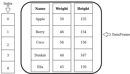
Let's create a DataFrame object called avatars with the contents shown below (the same data in the figure earlier):
| Name | Weight | Height |
|---|---|---|
| Apple | 50 | 155 |
| Berry | 46 | 154 |
| Coco | 56 | 156 |
| Dunkin | 44 | 167 |
| Ella | 45 | 150 |
For a small table like this, we can create the object by calling pandas.DataFrame() with a nested list as its first argument.
"""Creates a DataFrame object from a list of lists (named `source_table` here).
Feed this as the first argument of `pandas.DataFrame` below.
Uncomment the code lines and run them""";

source_table = [ ['Apple', 50, 155],
                 ['Berry', 46, 154],
                 ['Coco', 56, 156],
                 ['Dunkin', 44, 167],
                 ['Ella', 45, 150] ]

#avatars = pandas.DataFrame(#TODO, columns=['Name', 'Weight', 'Height'])
#print(avatars)
NOTES:
- By default, an integer sequence (
0,1,2, ...) is used as the labels (index). This can be overriden by theindex=argument. - Specifying column names is optional; if not given, the default of an integer sequence will also be used.
- Jupyter can display a
DataFramevariable in a nice format by simply mentioning the variable name as the last line of a code cell. For example, typeavatarsin the cell below and run it:
"""Type `avatars` (no quotes) and run the cell""";
#TODO
3.1.2 How Big is My Data?
Let's learn how to know the sizes, columns, index, and data types of a DataFrame object.
Use the len function to get the number of rows (records) in a DataFrame:
"""Inquire the number of rows in `avatars`""";
#print(#TODO)
Get the number of rows and columns using the shape attribute:
print(avatars.shape)
The shape attribute yields a tuple of two numbers:
the number rows and the number of columns.
Use the subscript operator [] to get the individual values:
"""Uncomment and modify to obtain the number of rows and columns""";
#print("The number of rows =", avatars.shape[0])
#print("The number of columns =", avatars.#TODO)
The index attribute yields the index, i.e. the collection of row labels:
"""Print the index of avatars:""";
#print(avatars.#TODO)
The names of the columns are given by the columns attribute:
print(avatars.columns)
Like shape, the individual elements in column can be accessed using the [] operator.
QUESTION: Print the name of the second column.
"""Make the following code print the name of the second column in df_mystery:""";
#print("The name of the second column is:", #TODO)
The dtypes attribute returns the data types associated with the columns:
"""Print the data types of the columns in avatars:""";
#print(avatars.#TODO)
We will discuss data types more later.
#BEGIN-OPTIONAL-SECTION
OPTIONAL: Is it a Series or a DataFrame?
At times we may want to know whether an object is a
Seriesor aDataFrame. Thetype()function tells the type of a Python object.QUESTION: Please find out the object type of
CPU_USAGEandavatars:
"""Uncomment and modify to print the type of CPU_USAGE variable""";
#print(#TODO(CPU_USAGE))
"""Now print the type of avatars""";
#TODO
#END-OPTIONAL-SECTION
3.1.3 Reading Data from a CSV File
When performing data analytics with pandas, data is usually read from an external file, instead of embedded in the notebook or the script.
This becomes an absolute necessity when handling large sizes of data.
The CSV format is frequently used with pandas because it is straightforward to make and comprehend.
It is a plain text file where each adjacent field is separated by a comma character.
pandas provides the pandas.read_csv() function to load data from a CSV file to a DataFrame.
As an example, in your current directory there is a file called avatars.csv.
Let's load this to a variable called avatars_read:
"""Uncomment and run the code below to load data from 'avatars.csv'.
   Replace #TODO with name of the data file.""";

#avatars_read = pandas.read_csv("#TODO")
#print(avatars_read)
QUESTION: Compare avatars_read with the previous DataFrame. Do they have the same contents?
How does pandas know the column names?
To answer that, let's inspect avatars.csv.
"""Use the UNIX `cat` command to print the contents of avatars.csv:""";
! cat avatars.csv
pandas.read_csv does a lot of work for you behind the scenes!
By default, it detects the names of the column from the first row of the table;
it also detects the data type of each column (numbers, strings, etc.).
3.2 Loading Sherlock Data
In the sherlock subdirectory, we have prepared a tiny subset of the Sherlock's "Application" dataset in a file named sherlock_mystery.csv.
Let us load that data into an object named df_mystery and print the contents.
IMPORTANT: Make sure that you read this data file at this point in order to do the subsequent exercises!
"""Edit and uncomment to load the Sherlock data file,
'sherlock/sherlock_mystery.csv' """;
#df_mystery = pandas.#TODO("#TODO")
"""Display the contents of df_mystery""";
#TODO
3.2.1 Initial DataFrame Exploration
When working with a new dataset, we always ask a lot of questions to familiarize ourselves with it. For example:
- How many columns and rows exist in this dataset?
- What columns are available in the dataset?
- What does the data look like? Can we learn some characteristics about the data?
QUESTIONS: Use the functions you've learned so far to answer the questions above.
"""Answer the questions above about the `df_mystery` dataset""";
# How many columns and rows?
#print(#TODO)
# What are the columns?
#print(#TODO)
# Examine the data; what are the data types?
#print(#TODO)
A DataFrame has a lot of handy methods and attributes which help us know our new dataset. Use attributes like shape, and methods like info, size, describe, head, tail.
The head and tail functions provide a handy way to print only a few records at the beginning and end of a DataFrame, respectively:
"""Uncomment and run to apply head() to df_mystery.
   How many rows get printed?""";
#df_mystery.head()
"""Print the first 10 rows of the DataFrame:""";
#print(df_mystery.#TODO(10))
Now experiment with the tail() function:
"""Modify the code to apply tail() to df_mystery. Optionally set the number of rows to display.""";
#df_mystery.#TODO(#TODO)
The describe() function provides the statistical information about all the numerical columns:
"""Apply describe() to df_mystery and observe the output:""";
#df_mystery.#TODO()
QUESTION: How many columns are in the describe() output above?
How many columns are in the original dataset?
NOTE: The non-numerical columns will be quietly ignored.
QUIZ: What is the mean value of num_threads?
71.36562.0000.075none of the above
The .T transpose operator would rotate the table by 90 degrees by swapping the rows and columns.
It can help us view a long horizontal table better:
"""Transpose the output of df_mystery.describe() use the .T operator:""";
#df_mystery.describe().#TODO
Pay attention to the mean, minimum, maximum values. These statistical numbers are worth taking time to digest, because they tell us a lot about the variation (distribution) of the values in each column.
The info() method prints a lot of useful information about a DataFrame object:
- the information about the index
- the information about every column (the name, the number of non-null elements, and the data type)
"""Apply the info() function and understand the result:""";
#df_mystery.#TODO()
The data types are quite important!
int64 refers to an integer (whole-number);
float64 refers to a real number;
object in the example above is used to contain text data (WhatsApp, Facebook).
We have learned that many of these information are given by the shape, columns, index, and dtypes attributes of the DataFrame object.
EXERCISE: If you haven't already, print these attributes and compare them with the
info()output above.
""" Do some exploration using `shape`, `columns`, etc.""";
#print(#TODO)
#print(#TODO)
3.3 Accessing Elements in a DataFrame
Similar to the Series object, the indexing operators [] and .loc[] can be used to access specific elements in a DataFrame object.
However, there are several forms, each accomplishing different purposes, as we shall learn now.
Let us create a small subset (6 rows) of the data so we don't see a deluge of data:
df6 = df_mystery.head(6).copy()
df6
3.3.1 Individual Column
The [] subscripting operator can provide access to an individual column:
"""Uncomment code and run, and observe the result:""";
#df6['ApplicationName']
QUESTION: From the output above, can you tell what type of object is returned?
Is it a DataFrame or a Series?
Explain the reason.
Hint: Use the type function to confirm:
"""Find out the object type of `df6[ApplicationName`]""";
#TODO
3.3.2 Multiple Columns
We can feed a list of column names into the [] operator to select multiple columns.
QUESTION: Select the following columns from the df6 object: ApplicationName, CPU_USAGE, num_threads. What type of object do you anticipate?
"""Uncomment and put in the appropriate column names per instruction above""";
#df6[[#TODO]]
3.3.3 Filtering Multiple Rows by Boolean
We can also feed an array of Boolean to the [] operator; but unlike the two previous uses, this will select rows (instead of columns) based on the Boolean values.
"""Uncomment and run the following codes; explain your observation""";

#df6_filt = df6[[True, False, False, True, True, False]]
#df6_filt
3.3.4 Selecting Row(s) by Labels
The .loc[] operator with a single argument is used to select DataFrame rows by the specified label(s). For example:
df6.loc[1]
Like before, since we specify only one row label as a scalar, this operation returns a Series object.
You can also return multiple rows by feeding it with the list of row labels, e.g.
"""Uncomment and run to select rows labeled 1, 3, 5""";
#df6.loc[[#TODO]]
3.3.5 Selecting Individual or Multiple Cell(s)
The .loc[] operator also supports a two-argument syntax to access one or more specific cells in the DataFrame, by specifying both the row and column labels--in that order.
In this fashion, this operator is akin to making cell references in a spreadsheet (such as A6, B20, etc.).
An example of selecting an individual cell at row label 1 and column named num_threads:
"""Uncomment and run to select an individual cell:""";
#print(df6.loc[1, 'num_threads'])
As in the [] operator, the row and/or column specification can be a list also to allow us to create a complex inquiry into the data, for example:
"""Uncomment the code below, select cells at the rows labeled [1,2,5]
and the following columns: ['num_threads', 'CPU_USAGE', 'ApplicationName']""";
#print(df6.loc[#TODO,#TODO])
A list of Boolean values can also be given to select the desired row(s) and/or column(s):
"""Uncomment and modify:
Pass on [False,True,True,False,True] as the row selector,
and select only two columns: 'num_threads' and 'CPU_USAGE'""";
#print(df6.loc[#TODO,#TODO])
QUESTION: The row selector is definitely too short (only 6 elements), whereas df_mystery has 200 rows.
What would happen to the rest of the rows if the length of the row selector is less than the number of rows of df_mystery?
Similar to the case of Series, the .loc[] operator can be used to update values in a DataFrame object, but the values returned by [] should generally be used as read-only.
QUESTION: Please update the value of CPU_USAGE for row labeled 2 to 0.01
"""Uncomment and modify to update the cell labeled [2, 'CPU_USAGE'] to a new value, 0.01""";
#df6.loc#TODO
3.3.6 Slicing Operator
In the indexing of rows and columns, the colon character (:) can be used in lieu of row or column label(s), and it will mean "everything" in that dimension.
QUESTION: Think first before doing! What does each expression below mean, and what will be the output?
df6.loc[1, :]
df6.loc[:, 'CPU_USAGE']
"""Use this cell to experiment and observe the output""";
The slicing operator also supports one or two endpoints. Here are several expressions to test:
df6.loc[:3]
df6.loc[3:]
df6.loc[2:5]
df6.loc[:3, 'CPU_USAGE']
df6.loc[:3, 'CPU_USAGE':'num_threads']
"""Uncomment code to run and observe the output""";
#df6.loc[:3]
df6.loc[3:]
df6.loc[:3, 'CPU_USAGE':'num_threads']
3.4 Data Access Exercises
EXERCISE 1: For each pair of commands below, what are the difference(s) within each pair?
(pair 1)
df_mystery['CPU_USAGE']
df_mystery[['CPU_USAGE']]
(pair 2)
df_mystery.loc[1]
df_mystery.loc[[1]]"""Use this code cell to experiment""";
EXERCISE 2: Extract a subset of df_mystery for rows labeled from 5 through 15 (inclusive endpoints), and include only columns from ApplicationName through priority.
"""Use this code cell to make your solution""";
EXERCISE 3: The first column named Unnamed: 0 seems to contain absurd data.
Using the indexing syntax we've learned here, create a new DataFrame that does not contain this column.
Hint: There are a few ways of doing this, but there is one syntax that is particularly compact. Be mindful of the position of that column.
"""Use this code cell to make your answer""";
# df_no_Unnamed = df_mystery#TODO
EXERCISE 4: Let's examine the data in df6 again.
The cminflt column does not contain any valid values (NaN means "not a number").
Suppose we know that zero is a safe default for cminflt.
Write the statement to set all the values in this column to zero.
Hint: In pandas, you can use a scalar assignment to assign one value to all the selected cells (columns, rows, or other selections): df.loc[...] = 0.0
"""Use this cell to make your solution""";
Please print df6 below here to confirm that you get the desired effect.
In case you mess up, re-initialize df6 using:
df6 = df_mystery.head(6).copy()before doing further testings.
df6
4 Making Sense of Data with Visualization
Visualization is a powerful tool to let us comprehend the data, because it readily gives us a broader perspective of the data compared to just staring at the numbers. In this section, we will introduce some basic visualization techniques to make sense of our mystery Sherlock dataset. A latter notebook will be dedicated to more in-depth visualization techniques.
4.1 Plotting Raw Data
Let us focus only on the vsize column of the df_mystery dataset.
pandas makes it very easy to plot the raw data, which we will compare to the descriptive statistics we've encountered earlier. The syntax to plot the values in a Series S (remember that a DataFrame column is a Series!) is: S.plot(kind='line').
QUESTION: Plot the values of vsize below:
"""Modify and uncomment to plot 'vsize'""";
#df_mystery[#TODO].plot(kind='line')
NOTES:
- The vertical tick labels are in the billions (that's the meaning of
1e9on the top left of the graph); - The horizontal tick labels are the row labels.
Now compare these values with descriptive statistics of the vsize column:
"""Modify and uncomment to print the statistics of 'vsize' column""";
#print(df_mystery['#TODO'].describe())
QUESTIONS:
- Take a look at the graph of
vsizeabove: what is the typical app's memory usage recorded in the df_mystery dataset? - Is that the typical value consistent with the output of the
describe()method above?
QUESTION: Create another plot for the CPU_USAGE field. What is the typical CPU usage of the apps? (Note: 100 means 100% busy CPU)
"""Create a line plot for `CPU_USAGE`""";
4.3 Box-and-Whisker Plot
Visualizing the descriptive statistics comes in handy when analyzing data. A box-and-whisker plot (often shortened "box plot") provides a concise, graphical depiction of the minimum, maximum, median, and quartiles of the values from a set of values. Khan academy has a tutorial video that explains all the parts of a box-and-whisker plot.
How to do this for the vsize column? Simply change the kind='line' to kind='box' in the plot statement above, and you're all set!
QUESTION: Draw the box-and-whisker plot for the vsize column and compare the result with the descriptive statistics above.
- Where is the median (
50%) in this graph? - Where are the
25%and75%percentiles in this graph? - Where are the
minandmaxin this graph?
"""Uncomment and modify to draw a box plot of the 'vsize' data""";

#df_mystery['#TODO'].plot(kind='box')
QUESTION: Compare the box plot above with the raw data plot produced earlier.
- Do the values look consistent?
- Does the descriptive statistics match the raw data?
4.4 Visualization with Seaborn
Seaborn visualization package can produce similar plots to what pandas alone can make, but with a much more robust set of capabilities and better aesthetics. Let's try an example here for the box plot:
"""Uncomment and modify to draw a box plot of 'vsize'""";

#seaborn.boxplot(x=df_mystery['#TODO'], color='cyan')
5. Summary & Further Resources
Pandas
Important Notes on DataFrame Indexing
In a DataFrame, the .loc[] operator is the only way to select specific row(s) by the labels, as the [] operator is reserved to select only column(s).
The .loc[] operator can also be used to write new values to particular location(s) in the DataFrame.
References & Cheatsheets
Our lesson page has a summary table of the commonly used indexing syntax.
pandas user's guide has a comprehensive documentation on selecting and indexing data.
pandas cheatsheet: https://pandas.pydata.org/Pandas_Cheat_Sheet.pdf
Please study these resources and keep them within easy reach. These are handy help when you are writing your own analysis pipeline using pandas.
Seaborn
To learn more about seaborn, please visit
Seaborn Tutorial.
Seaborn also has a
gallery of examples
to demonstrate what can be done with this package.
There are many sample codes to get your own visualizations started.
Common Conventions
It is a common practice for Python programmers to shorten module names:
pdforpandasnpfornumpypltformatplotlib.pyplotsnsforseaborn
At the beginning of a script or a notebook, they will declare:
import pandas as pd
import numpy as np
from matplotlib import pyplot as plt
import seaborn as sns
DataFrame variables often have df in its name---whether
df, df2, df_mystery, mystery_df, ....
The df part gives people a visual cue that the variable is a DataFrame object.